2 - Spatial data modelling: computer representations
Explain and be able to apply basic vector and raster spatial data structures including selecting a suitable data structure for geographic phenomena (level 1, 2 and 3).
Concepts
-
Line representation
Line data are used to represent one-dimensional objects such as roads, railroads, canals, rivers and power lines. Again, there is an issue of relevance for the application and the scale that the application requires.
For the example of mapping tourist information, bus, subway and tram routes are likely to be relevant line features. Some cadastral systems, on the other hand, may consider roads to be two-dimensional features, i.e. having a width as well as length. Previously, we noted that arbitrary, continuous curvilinear features are as equally difficult to represent as continuous fields. GISs, therefore, approximate such features (finitely!) as lists of nodes: the two end nodes and zero or more internal nodes, or vertices, define a line. Other terms for “line” that are commonly used in some GISs are polyline, arc or edge. A node or vertex is like a point, but it only serves to define the line and provide shape in order to obtain a better approximation of the actual feature. The straight parts of a line between two consecutive vertices or end nodes are called line segments. Many GISs store a line as a sequence of coordinates of its end nodes and vertices, assuming that all its segments are straight. This is usually good enough, as cases in which a single straight line segment is considered an unsatisfactory representation can be dealt with by using multiple (smaller) line segments, instead of one.
Still, in some cases we would like to have the opportunity to use arbitrary curvilinear features to represent real-world phenomena. Think of a garden design with perfectly circular or elliptical lawns, or of detailed topographic maps showing roundabouts and the sidewalks. In principle all of this can be stored in a GIS, but currently many systems do not accommodate such shapes. A GIS function supporting curvilinear features uses parameterized mathematical descriptions, a discussion of which is beyond the scope of this textbook. Collections of (connected) lines may represent phenomena that are best viewed as networks. With networks, interesting questions arise that have to do with connectivity and network capacity. These relate to applications such as traffic monitoring and watershed management. With network elements—i.e. the lines that make up the network—extra values are commonly associated, such as distance, quality of the link or the carrying capacity.
-
Topological data model
The boundary model is an improved representation that deals with the disadvantages of the naive polygon which is described in polygons. It stores parts of a polygon’s boundary as non-looping arcs and indicates which polygon is on the left and which is on the right of each arc. A simple example of the boundary model can be seen below. It illustrates which additional information is stored about spatial relationships between lines and polygons. Obviously, real coordinates for nodes (and vertices) will also be stored in another table. The boundary model is also called the topological data model as it captures some topological information, such as polygon neighbourhood, for example. You can read more about topological information in Topology. Observe that it is a matter of a simple query to find all the polygons that are the neighbour of a given polygon, unlike the case above.
-
Time
As time is the central concept of the temporal dimension, a brief examination of the nature of time may clarify our thinking when we work with this dimension:
- Discrete and continuous time: Time can be measured along a discrete or continuous scale. Discrete time is composed of discrete elements (seconds, minutes, hours, days, months, or years). For continuous time, no such discrete elements exist: for any two moments in time there is always another moment in between. We can also structure time by events (moments) or periods (intervals). When we represent intervals by a start and an end event, we can derive temporal relationships between events and periods, such as “before”, “overlap”, and “after”.
- Valid time and transaction time: Valid time (or world time) is the time when an event really happened, or a string of events took place. Transaction time (or database time) is the time when the event was stored in the database or GIS. Note that the time at which we store something in a database is typically (much) later than when the related event took place.
- Linear, branching and cyclic time: Time can be considered to be linear, extending from the past to the present (‘now’), and into the future. This view gives a single time line. For some types of temporal analysis, branching time - in which different time lines from a certain point in time onwards are possible - and cyclic time - in which repeating cycles such as seasons or days of the week are recognized - make more sense and can be useful.
- Time granularity: When measuring time, we speak of granularity as the precision of a time value in a GIS or database (e.g. year, month, day, second). Different applications may obviously require different granularity. In cadastral applications, time granularity might well be a day, as the law requires deeds to be date-marked; in geological mapping applications, time granularity is more likely to be in the order of thousands or millions of years.
- Absolute and relative time: Time can be represented as absolute or relative. Absolute time marks a point on the time line where events happen (e.g. “6 July 1999 at 11:15 p.m.”). Relative time is indicated relative to other points in time (e.g. “yesterday”, “last year”, “tomorrow”, which are all relative to “now”, or “two weeks later”, which is relative to some other arbitrary point in time.).
-
Regular Tessellation
A regular tessellation is a partitioning of space into mutually exclusive cells that together make up the complete study area and in which the cells have the same shape and size. A simple example of this is a rectangular raster of unit squares, represented in a computer in the 2D case as an array of n x m elements.
-
Spatial data layer
A spatial data layer is either a representation of a continuous or discrete field, or a collection of objects of the same kind. The main principle of data organization applied in a GIS is that of spatial data layers. Usually, the data are organized such that similar elements are in a single data layer (Figure 1). For example, all telephone booth point objects would be in one layer, and all road line objects in another. A data layer contains spatial data, as well as attribute (i.e. thematic) data, which further describes the field or objects in the layer. Attribute data are quite often arranged in tabular form, maintained in some kind of geo-database.
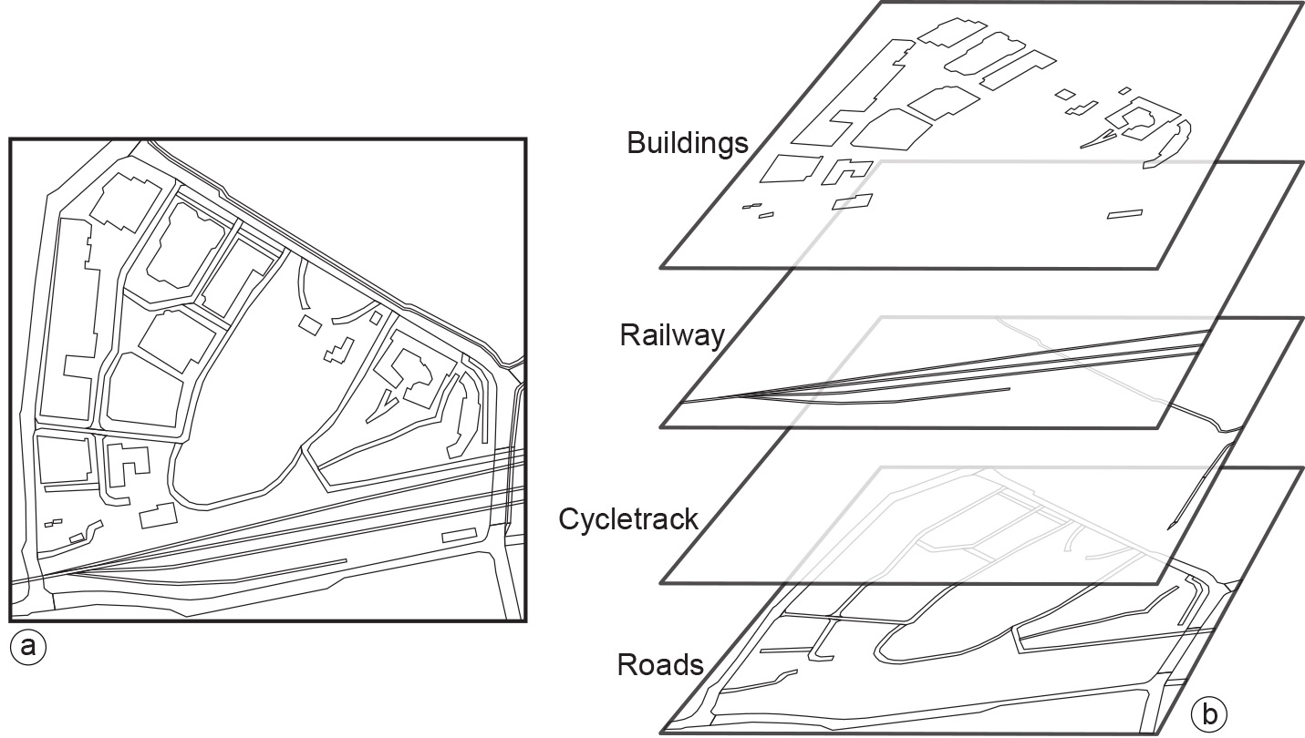
Figure 1: Various objects displayed as area objects in a vector representation. Similar data types are stored in the same single layer (e.g. Buildings). For each different type a new layer is used (b). -
Data storage and maintainance
The way that data are stored plays a central role in their processing and, eventually, our understanding of them. In most available systems, spatial data are organized in layers by theme and/or scale. Examples are layers of thematic categories, such as land use, topography and administrative subdivisions, each according to their mapping scale. An important underlying principle is that a representation of the real world has to be designed such that it reflects phenomena and their relationships as naturally as possible. In a GIS, features are represented together with their attributes—geometric and non-geometric—and relationships. The geometry of features is represented with primitives of the respective dimension: a windmill probably as a point; an agricultural field as a polygon. The primitives follow either the vector or the raster approach.
Vector data types describe an object through its boundary, thus dividing the space into parts that are occupied by the respective objects. The raster approach subdivides space into (regular) cells, mostly as a square tessellation of two or three dimensions. These cells are called pixels in 2D and voxels in 3D. The data indicate for every cell which real-world feature is covered, provided the cell represents a discrete field. In the case of a continuous field, the cell holds a representative value for that field. The Table below lists advantages and disadvantages of raster and vector representations.
Table: Raster and vector representations compared Raster representation Vector representation Advantages Advantages ∙ simple data structure ∙ efficient representation of topology ∙ simple implementation of ∙ adapts well to scale changes overlays ∙ allows representing networks ∙ efficient for image processing ∙ allows easy association with attribute data disadvantages Disadvantages ∙ less compact data structure ∙ complex data structure ∙ difficulties in representing ∙ overlay more difficult to implement topology ∙ inefficient for image processing ∙ cell boundaries independent ∙ more update-intensive of feature boundaries The storage of a raster is, in principle, straightforward. It is stored in a file as a long list of values, one for each cell, preceded by a small list of extra data (the “file header”), which specifies how to interpret the long list. The order of the cell values in the list can, but need not necessarily, be left to right, top to bottom. This simple encoding scheme is known as row ordering. The header of the raster will typically specify how many rows and columns the raster has, which encoding scheme was used, and what sort of values are stored for each cell.
Raster files can be large. For efficiency reasons, it is wise to organize the long list of cell values in such a way that spatially nearby-cells are also near to each other in the list. This is why other encoding schemes have been devised. The reader is referred to Laurrini and Thompson (1992) for a more detailed discussion.
Low-level storage structures for vector data are much more complicated, and a discussion of this topic is beyond the scope of this textbook. The best intuitive understanding can be obtained from Topological Data Model, which illustrates a boundary model for polygon objects. Similar structures are in use for line objects. For further, advanced, reading see Samet(1990). GIS packages support both spatial and attribute data, i.e. they accommodate spatial data storage using a vector approach and attribute data using tables. Historically, however, database management systems (DBMSs) have been based on the notion of tables for data storage.
GIS applications have been able to link to an external database to store attribute data and make use of its superior data management functions. Currently, all major GIS packages provide facilities to link with a DBMS and exchange attribute data with it. Spatial (vector) and attribute data are still sometimes stored in separate structures, although they can now be stored directly in a spatial database. Maintenance of data, spatial or otherwise, can best be defined as the combination of activities needed to keep the data set up to date and as supportive as possible for the user community. It deals with obtaining new data and entering them into the system, as well as possibly replacing outdated data. The purpose is to have an up-to-date, stored data set available. After a major flood, for instance, we may have to update road-network data to reflect that roads have been washed away or have become otherwise impassable.
The need for updating spatial data originates from the requirements posed by the users, as well as the fact that many aspects of the real world change continuously. Data updates can take different forms. It may be that a completely new survey has been carried out, from which an entirely new data set will be derived, to replace the current set. This is typically the case if the spatial data originate from remote sensing, for example, from a new vegetation-cover set or from a new digital elevation model. Furthermore, local ground surveys may reveal local changes, such as new constructions or changes in land use or ownership. In such cases, local changes to a large spatial data set are typically required. Such local changes should take into account matters of data consistency, i.e. they should leave other spatial data within the same layer intact and correct.
-
Vector Representation
Tessellations do not explicitly store georeferences of the phenomena they represent. A georeference is a coordinate pair from some geographic space, and is also known as a vector. Instead, tesselations provide a georeference of the lower left corner of the raster, for instance, plus an indicator of the raster’s resolution, thereby implicitly providing georeferences for all cells in the raster. In vector representations, georeferences are explicitly associated with the geographic phenomena.
-
Irregular Tessellation
Irregular Tessellations are partitions of space into mutually distinct cells, but now the cells may vary in size and shape, allowing them to adapt to the spatial phenomena that they represent. Irregular tessellations are more complex than regular ones, but they are also more adaptive, which typically leads to a reduction in the amount of computer memory needed to store the data.
Regular tessellations provide simple structures with straightforward algorithms that are, however, not adaptive to the phenomena they represent. This means they might not represent the phenomena in the most efficient way. For this reason, substantial research effort has been put into irregular tessellation.
-
Tessellation
Tessellation (or tiling) is a partitioning of space into mutually exclusive cells that together make up the complete study space. For each cell, a (thematic) value is assigned to characterize that part of space. There are regular and irregular tessellations.
In a regular tessellation, the cells have the same shape and size; a simple example of this is a rectangular raster of unit squares, represented in a computer in the 2D case as an array of n × m elements. These tessellations are known under various names in different GIS packages: Rasters or raster map. The size of the area that a single raster cell represents is called the raster's resolution.
Irregular Tessellation are partitions of space into mutually distinct cells, but now the cells may vary in size and shape, allowing them to adapt to the spatial phenomena that they represent.
-
Node
Two end nodes and zero or more internal nodes, or vertices, define a line. A node or vertex is like a point, but it only serves to define the line and provide shape in order to obtain a better approximation of the actual feature. The straight parts of a line between two consecutive vertices or end nodes are called line segments. Many GISs store a line as a sequence of coordinates of its end nodes and vertices, assuming that all its segments are straight.
-
Point representation
Points are defined as single coordinate pairs (x, y) in 2D space, or coordinate triplets (x, y, z) in 3D space. Points are used to represent objects that are best described as shapeless, size-less, zero-dimensional features. Whether this is the case really depends on the purposes of the application and also on the spatial extent of the objects compared to the scale used in the application. For a tourist map of a city, a park would not usually be considered a point feature, but perhaps a museum would, and certainly a public phone booth might be represented as a point. In addition to the georeference, administrative or thematic data are usually stored for each point object that can capture relevant information about it. For phone-booth objects, for example, this may include the telephone company owning the booth, its phone number and the date it was last serviced.
-
Area representation
When area objects are stored using a vector approach, the usual technique is to apply a boundary model. This means that each area feature is represented by some arc/node structure that determines a polygon as the area’s boundary. A polygon representation for an area object is another example of a finite approximation of a phenomenon that may have a curvilinear boundary in reality.
-
Resolution
Resolution describes the ability to resolve small details (in space, time or the electromagnetic spectrum). When applied to spatial data, the term resolution is commonly associated with the cell width of the tessellation applied.
-
Spatial-Temporal data model
The way we represent relevant components of the real world in our models determines the kinds of questions we can or cannot answer. We have already discussed representation issues for spatial features, but so far we have ignored issues for incorporating time. The main reason is that GISs still offer limited support for doing so. As a result, most studies require substantial efforts from the GIS user in data preparation and data manipulation. Also, besides representing an object or field in 2D or 3D space, the temporal dimension is of a continuous nature. Therefore, in order to represent it in a GIS we have to discretize the time dimension.
Spatio-temporal data models are ways of organizing representations of space and time in a GIS. Several representation techniques have been proposed in the literature. Perhaps the most common of these is the “snapshot state”, which represents a single moment in time of an ongoing natural or man-made process. We may store a series of these “snapshot states” to represent “change”, but we must be aware that this is by no means a comprehensive representation of that process. Further treatment of spatio-temporal data models is outside the scope of this book and readers are referred to Langran (1992) for a discussion of relevant concepts and issues.
-
Geographical representation
A geographical representation considers the way geoinformation, such as fields and objects, are represented in computers.
A geographic field can be represented by means of a tessellation, a TIN or a vector representation. The choice between them is determined by the requirements of the application in mind. It is more common to use tessellations, notably rasters, for field representation, but vector representations are in use too.
The representation of geographic objects is most naturally supported with vectors. After all, objects are identified by the parameters of location, shape, size and orientation, and many of these parameters can be expressed in terms of vectors.
-
Temporal attribute
Besides having geometric, thematic and topological properties, geographic phenomena also change over time and are thus dynamic phenomena. Examples include identifying the owners of a land parcel in 1972, or determining how land cover in a certain area changed from native forest to pasture land over a specific time period. Some features or phenomena change slowly, e.g. geological features or land cover, as in the example just given. Other phenomena change very rapidly, such as the movement of people or atmospheric conditions. For an increasing number of applications, these changes themselves are the key aspect of the phenomenon to be studied. For different applications, different scales of measurement will apply.
-
Where and when did something happen?
-
How fast did this change occur?
-
In which order did the changes occur?
-
-
Triangulated Irregular Networks
Triangulated Irregular Networks (TINs) is a commonly-used data structure in GIS software. It is a standard implementation techniques for digital terrain models, but it can also be used to represent any continuous field. The principles on which a TIN is based are simple. It is built from a set of locations for which we have a measurement, for instance an elevation. The locations can be arbitrarily scattered in space and are not usually on a regular grid. Any location together with its elevation value can be viewed as a point in three-dimensional space. From these 3D points, we can construct an irregular tessellation made of triangles.
-
Map scale
In the practice of spatial data handling, one often comes across questions like “What is the resolution of the data?” or “At what scale is your data set?” Now that we have moved firmly into the digital age, these questions sometimes defy an easy answer. Map scale can be defined as the ratio between the distance on a printed map and the distance of the same stretch in the terrain.
A 1:50,000 scale map means that 1 cm on the map represents 50,000 cm (i.e. 500 m) in the terrain. “Large-scale” means that the ratio is relatively large, so typically it means there is much detail to see, as on a 1:1000 printed map. “Small-scale”, in contrast, means a small ratio, hence less detail, as on a 1:2,500,000 printed map.
-
Data integration
Combination of Earth observation data with other types of geospatial data is highly recommended since existing information can be essential for improving the interpretation of remote sensing data. The automatic classification of agricultural crops from multispectral image data is such an example. Pixel-by-pixel classification usually gives many errors, owing to sensor noise and field heterogeneity. However, if parcel boundaries are known from a GIS database, one can classify all pixels within a field as a group, which reduces the number of misclassifications enormously, provided, of course, that the group as a whole is correctly classified.
Data can be integrated in an almost infinite number of ways. Results from data integration can, again, be combined with other geospatial data to produce yet other new information, and so on.