Geographic object

When a geographic phenomenon is not present everywhere in the study area, but somehow “sparsely” populates it, we look at it as a collection of geographic objects. Such objects are usually easily distinguished and named, and their position in space is determined by a combination of one or more of the following parameters:

• location (where is it?)
• shape (what form does it have?)
• size (how big is it?)
• orientation (in which direction is it facing?).

How we want to use the information determines which of these four parameters is required to represent the object. For instance, for geographic objects such as petrol stations all that matters in an in-car navigation system is where they are. Thus, in this particular context, location alone is enough, and shape, size and orientation are irrelevant. For roads, however, some notion of location (where does the road begin and end?), shape (how many lanes does it have?), size (how far can one travel on it?) and orientation (in which direction can one travel on it?) seem to be relevant components of information in the same system.

Shape is an important component because one of its factors is dimension. This relates to whether an object is perceived as a point feature or a linear, area or volume feature. In the above example, petrol stations are apparently zero-dimensional, i.e. they are perceived as points in space; roads are one-dimensional, as they are considered to be lines. In another use of road information - for instance, in multi-purpose cadastral systems, in which the precise location of sewers and manhole covers matters - roads might be considered as two-dimensional entities, i.e. as areas.

Figure 1 illustrates geological faults in the Falset study area, a typical example of a geographic phenomenon that is made up of objects. Each of the faults has a location, and the fault’s shape is represented as a one-dimensional object. The size, which is length in the case of one-dimensional objects, is also indicated. Orientation does not play a role here.

Usually, we do not study geographic objects in isolation, but instead look at collections of objects, which we consider as a unit. These collections may have specific geographic characteristics. Most of the more interesting ones obey specific natural laws. The most common (and obvious) of these characteristics is that different objects do not occupy the same location. This, for instance, holds for the collection of petrol stations in an in-car navigation system, the collection of roads in that system, and the collection of land parcels in a cadastral system. This natural law of “mutual non-overlap” has been a guiding principle in the design of computer representations of geographic phenomena.

Collections of geographic objects can also be interesting phenomena at a higher level of aggregation: forest plots form forests, groups of parcels form suburbs, streams, brooks and rivers form a river drainage system, roads form a road network, and SST buoys form an SST sensor network. It is sometimes useful to view geographic phenomena at this more aggregated level and look at characteristics such as coverage, connectedness and capacity. For example:

• Which part of a particular road network is within 5 km of a petrol station (a coverage question)?

• What is the shortest route between two cities via the road network (a connectedness question)?

• How many cars can optimally travel from one city to another in an hour (a capacity question)?

In this context, multi-scale approaches are sometimes used. Such approaches deal with maintaining, and operating on, multiple representations of the same geographic phenomenon, e.g. a point representation in some cases, and an area representation in others. To support these approaches, the database must store representations of geographic phenomena (spatial features) in a scaleless and seamless manner. Scaleless means that all coordinates are world coordinates, i.e. are given in units that are used to reference features in the real world (using a spatial reference system). From such values, calculations can be easily performed and an appropriate scale can be chosen for visualization. Other spatial relationships between the members of a collection of geographic objects may exist and can be relevant in GIS usage. Many of these fall under the category of topological relationships.

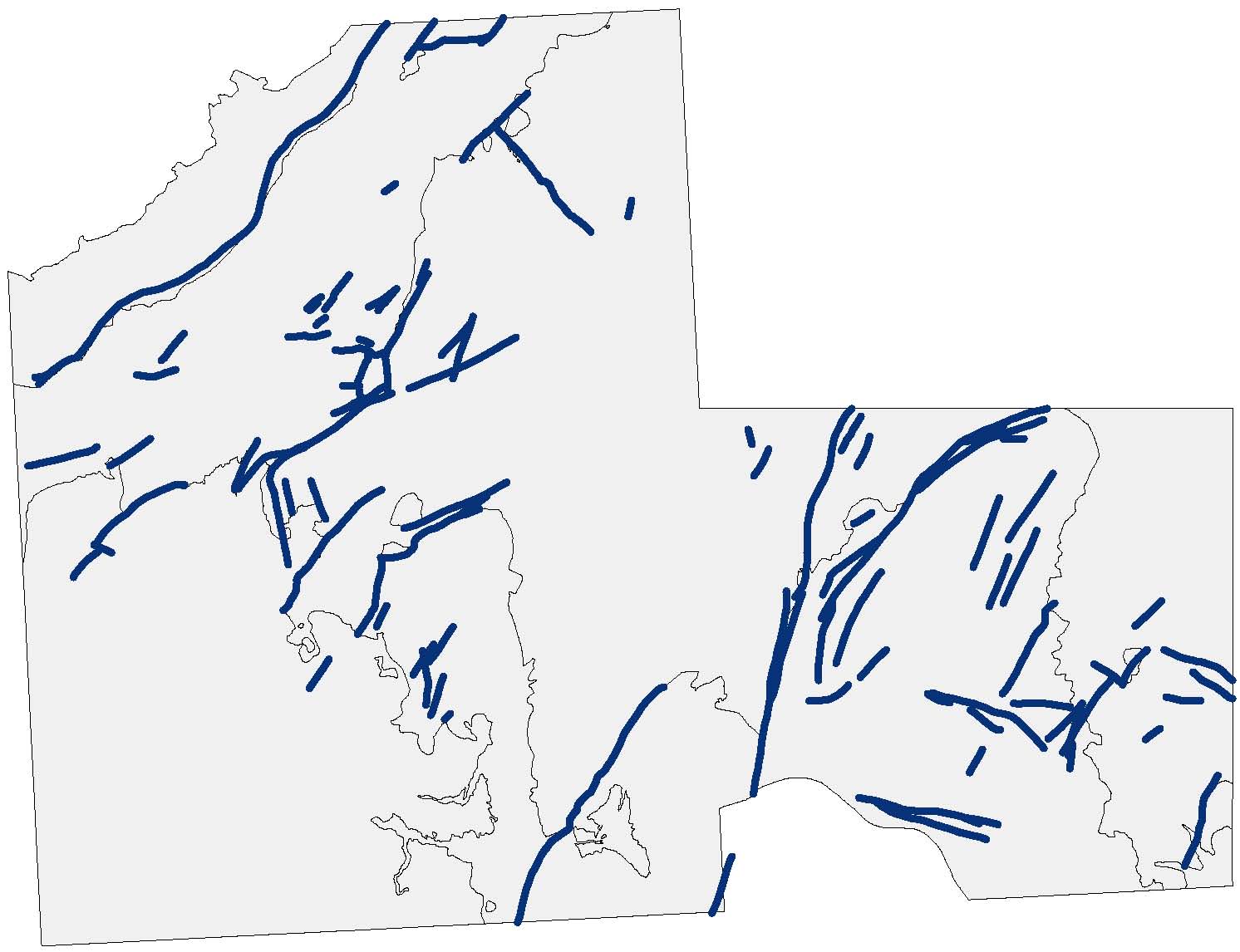
A number of geological faults in the Falset (Spain) study area. Faults are indicated as blue lines; the study area, with main geological eras, is indicated by the grey background only as a reference.

The representation of geographic objects is most naturally supported with vectors. After all, objects are identified by the parameters of location, shape, size and orientation, and many of these parameters can be expressed in terms of vectors. Tessellations are also commonly used for representing geographic objects.

Tessellations for representing geographic objects

Remotely-sensed images are an important data source for GIS applications. Unprocessed digital images contain many pixels, each of which carrying a reflectance value. Various techniques exist to process digital images into classified images that can be stored in a GIS as a raster. Image classification characterizes each pixel into one of a finite list of classes, thereby obtaining an interpretation of the contents of the image. The recognized classes can be crop types, as in the case of Figure 2, or urban land use classes, as in the case of Figure 3. These figures illustrate the unprocessed images (a) and a classified version of the image (b). For the application at hand, perhaps only potato fields (Figure 2b, in yellow) or industrial complexes (Figure 3b, in orange) are of interest. This would mean that all other classes are considered unimportant and would probably be ignored in further analysis. If that further analysis can be carried out with raster data formats, then there is no need to consider vector representations.

Nonetheless, we must make a few observations regarding the representation of geographic objects in rasters. Line and point objects are more awkward to represent using rasters. Area objects, however, are conveniently represented in a raster, although area boundaries may appear as jagged edges. This is a typical by-product of raster resolution versus area size, and artificial cell boundaries. This may have consequences for area-size computations: the precision with which the raster defines the object’s size is limited. After all, we could say that rasters are area based and that geographic objects  that are perceived as lines or points are considered to have zero area size. Standard classification techniques may, moreover, fail to recognize these objects as points or lines.

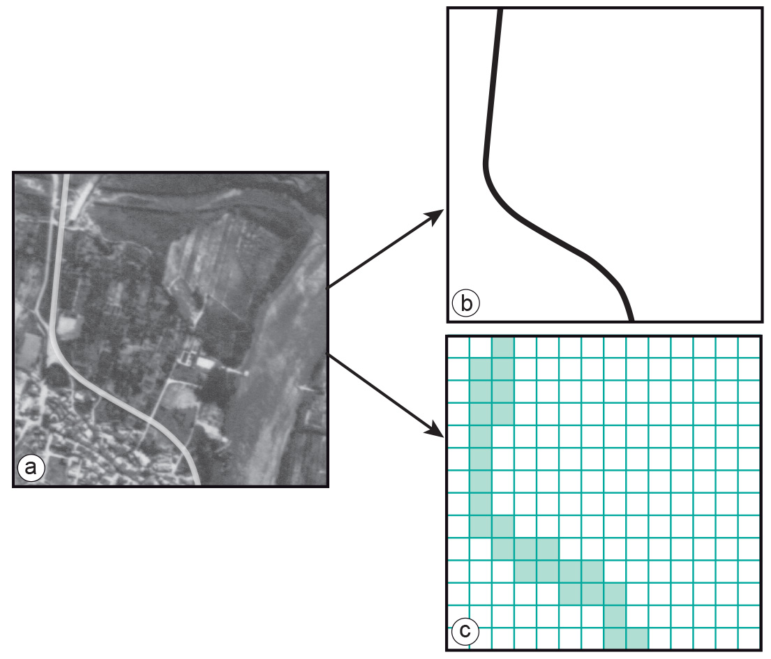
Many GISs support line representations in a raster, as well as operations on them. Lines can be represented as strings of neighbouring raster cells of equal value (Figure 4). Supported operations are connectivity operations and distance computations. Note that the issue of the precision of such computations needs to be addressed.

Vector representations of geographic objects

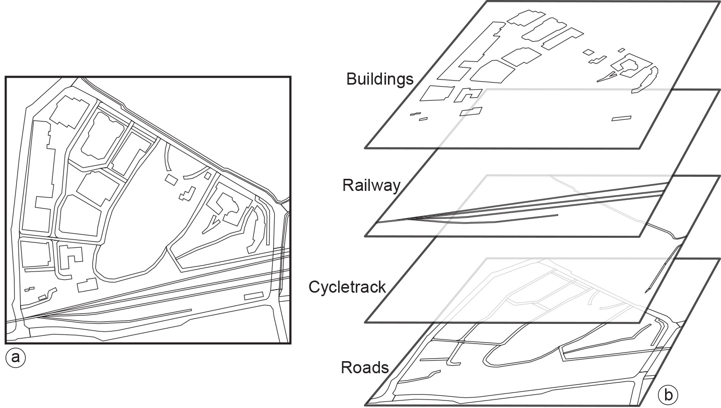
A more natural way of depicting geographic objects is by means of vector representations. Figure 5 shows a number of geographic objects in the vicinity of the ITC building. These objects are area representations in a boundary model. Nodes and vertices of the polylines that make up the objects’ boundaries are not illustrated, though obviously they have been stored.