Geographic field

A geographic field is a geographic phenomenon that has a value “everywhere” in the study area. We can therefore think of a field as a mathematical function f that associates a specific value with any position in the study area. Hence if (x, y) is a position in the study area, then f(x, y) expresses the value of f at location (x, y). Fields can be discrete or continuous.

In a discrete field, the study area is divided in mutually exclusive, bounded parts, with all locations in one part having the same field value.

In a continuous field, the underlying function is assumed to be “mathematically smooth”, meaning that the field values along any path through the study area do not change abruptly, but only gradually.

A geographic field can be represented by means of a tessellation, a TIN or a vector representation. The choice between them is determined by the requirements of the application in mind. It is more common to use tessellations, notably rasters, for field representation, but vector representations are in use too.

Raster representation of a field

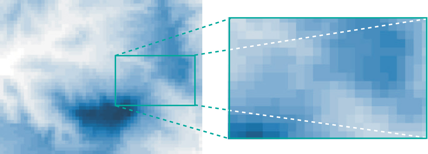
Figure 1 illustrates how a raster represents a field, in this case elevation. Different shades of blue indicate different elevation values, with darker blue tones indicating higher elevations. The choice of a blue spectrum is only to make the illustration aesthetically pleasing; real elevation values are stored in the raster, so we could have printed a real number value in each cell instead. This would not have made the figure very legible, however. A raster can be thought of as a long list of field values: actually, there should be m× n such values present. The list is preceded with some extra information, such as a single georeference for the origin of the whole raster, a cell-size indicator, the integer values for m and n, and an indicator of data type for interpreting cell values. Rasters and quadtrees do not store the georeference of each cell, but infer it from the extra information about the raster. A TIN is a much “sparser” data structure: as compared to a regular raster, the amount of data stored is less for a structure of approximately equal interpolation error. The quality of the TIN depends on the choice of anchor points, as well as on the triangulation built from it. It is, for instance, wise to perform “ridge following” during the data acquisition process for a TIN. Anchor points on elevation ridges will assist in correctly representing peaks and faces of mountain slopes.

Vector representation of a field

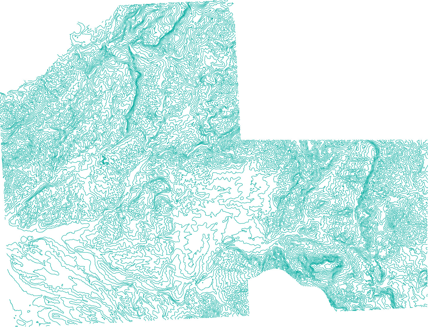
We briefly mention the vector representation for fields such as elevation, which uses isolines of the field. An isoline is a linear feature that connects points with equal field values. When the field is elevation, we also speak of contour lines. Elevations in the Falset study area are represented by contour lines in Figure 2. Both TINs and isoline representations use vectors. Isolines as a representation mechanism are not common, however. They are used as a geoinformation visualization technique (in mapping, for instance), but usually it is better to choose a TIN for representing this type of field. Many GIS packages provide functions to generate an isoline visualization from a TIN.