11 - Spatial analysis: classes of functions
Classify and explain spatial analysis functions (measurements, classification, overlay, neighbourhood and connectivity) in a raster and vector environment (level 1 and 2).
Concepts
-
Analysis
Analytical capabilities of a
GIS make use of spatial and non-spatial (attribute) data to answer questions and solve problems that are of spatial relevance. We now make a distinction between analysis (or analytical operations) and analytical models (often referred to as “modelling”). And by analysis we actually mean only a subset of what is usually implied by the term: we do not specifically deal with advanced statistical analysis (such as cluster detection or geostatistics).Analysis of spatial data can be defined as computing new information to provide new insights from existing spatial data. Consider an example from the domain of road construction. In mountainous areas, this is a complex engineering task with many cost factors, including the number of tunnels and bridges to be constructed, the total length of the tarmac, and the volume of rock and soil to be moved. GISs can help to compute such costs on the basis of an up-to-date digital elevation model and a soil map.The exact nature of the analysis will depend on the application requirements, but computations and analytical functions can operate on both spatial and non-spatial data.
-
Selection by attribute conditions
It is also possible to select features by using selection conditions on feature attributes. These conditions are formulated in SQL (if the attribute data reside in a relational database) or in a software-specific language (if the data reside in the GIS itself). This type of selection answers questions like “Where are the features with …?”
-
Query
When exploring a spatial data set, the first thing one usually wants to do is select certain features, to (temporarily) restrict the exploration. Such selections can be made on geometric/spatial grounds or on the basis of attribute data associated with the spatial features.
Selection conditions on attribute values can be combined using logical connectives such as AND, OR and NOT. Other techniques of selecting features can also usually be combined. Any set of selected features can be used as the input for a subsequent selection procedure. This means, for instance, that we can select all medical clinics first, then identify roads within 200 m of them, then select from those only the major roads, then select the nearest clinics to these remaining roads as the ones that should receive our financial support for maintenance. In this way, we are combining various techniques of selection.
Interactive Spatial Selection
In interactive spatial selection , one defines the selection condition by pointing at or drawing spatial objects on the screen display, after having indicated the spatial data layer(s) from which to select features. The interactively defined objects are called the selection objects; they can be points, lines, or polygons. The GIS then selects the features in the indicated data layer(s) that overlap (i.e. intersect, meet, contain, or are contained in;) with the selection objects. These become the selected objects.
Interactive spatial selection answers questions like “What is at …?” IN the Figure below, the selection object is a circle and the selected objects are the blue polygons; they overlap with the selection object.
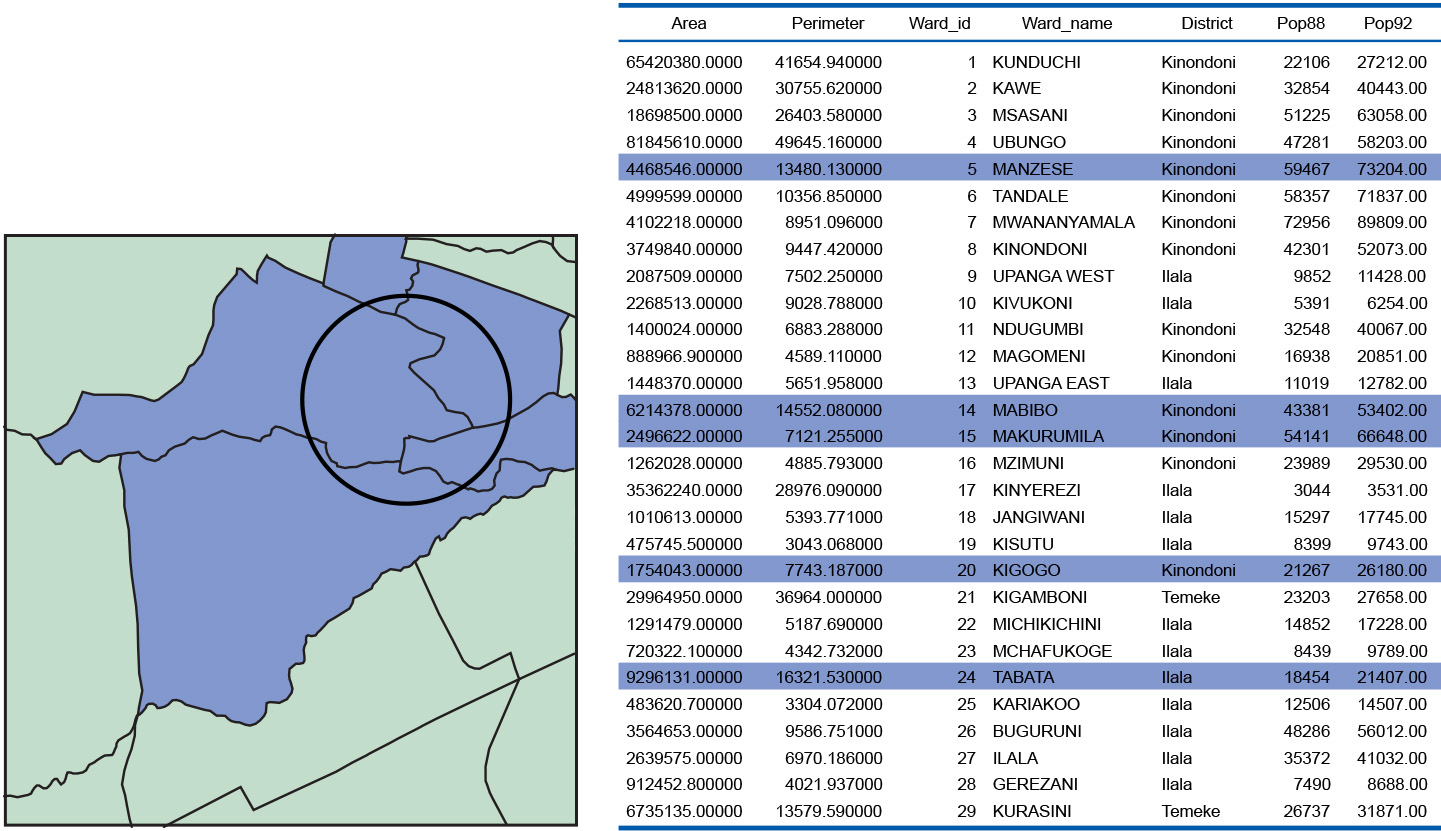
Figure: All city wards that overlap with the selection object—here a circle—are selected (left), and their corresponding attribute records are highlighted (right; only part of the table is shown). Data from an urban application in Dar es Salaam, Tanzania. -
Automatic reclassification
User-controlled classifications require a classification table or user interaction.
GIS software can also perform automatic classification, in which a user only specifies the number of classes in the output data set. The system automatically determines the class break points. The two main techniques of determining break points being used are the equal interval technique and the equal frequency technique.Equal Interval Technique
The minimum and maximum values vmin and vmax of the classification parameter are determined and the (constant) interval size for each category is calculated as (vmax - vmin) ∕ n, where n is the number of classes chosen by the user. This classification is useful in that it reveals the distribution pattern, as it determines the number of features in each category.
Equal Frequency Technique
This technique is also known as quantile classification. The objective is to create categories with roughly equal numbers of features per category. The total number of features is determined first, then, based on the required number of categories, the number of features per category is calculated. The class break points are then determined by counting off the features in order of classification parameter value.
-
Buffer
The principle of buffer zone generation is simple: we select one or more target locations and then determine the area around them within a certain distance.
In some case studies, zoned buffers must be determined, for instance in assessments of the effects of traffic noise. Most
GIS s support this type of zoned-buffer computation. An illustration is provided in Figure b of the Examples.In vector-based buffer generation, the buffers themselves become polygon features, usually in a separate data layer, that can be used in further spatial analysis. Buffer generation on rasters is a fairly simple function. The target location or locations are always represented by a selection of the raster’s cells and geometric distance is defined using cell resolution as the unit. The distance function applied is the Pythagorean distance between the cell centres. The distance from a non-target cell to the target is the minimal distance one can find between that non-target cell and any target cell.
Buffer generation on rasters is a fairly simple function. The target location or locations are always represented by a selection of the raster’s cells and geometric distance is defined using cell resolution as the unit. The distance function applied is the Pythagorean distance between the cell centres. The distance from a non-target cell to the target is the minimal distance one can find between that non-target cell and any target cell.
-
Surface Analysis
Continuous fields have a number of characteristics not shared by discrete fields. Since the field changes continuously, we can talk of slope angle, slope aspect and concavity/convexity of the slope.
These notions are not applicable to discrete fields. The discussions in this subsection use terrain elevation as the prototype example of a continuous field, but all aspects discussed are equally applicable to other types of continuous fields. Nonetheless, we regularly refer to the continuous field representation as a DEM, to conform with the most common situation.
-
Raster Proximity
Buffer generation on rasters is a fairly simple function. The target location or locations are always represented by a selection of the raster’s cells and geometric distance is defined using cell resolution as the unit. The distance function applied is the Pythagorean distance between the cell centres. The distance from a non-target cell to the target is the minimal distance one can find between that non-target cell and any target cell.
-
Measurement
Geometric measurement on spatial features includes counting, distance and area size computations. Here we discuss such measurements in a planar spatial reference system. We limit ourselves to geometric measurements and do not include attribute data measurement, which is typically performed in a database query language. Measurements on vector data are more advanced (and thus also more complex) than those on raster data.
-
Neighbourhood operations
Neighbourhood functions evaluate the characteristics of an area surrounding a feature’s location. A neighbourhood function “scans” the neighbourhood of the given feature(s), and performs a computation on it(them).
-
Proximity computations:
-
Buffer zone generation (or buffering) is one of the best-known neighbourhood functions. It determines a spatial envelope (buffer) around a given feature or features. The buffer created may have a fixed width or a variable width that depends on characteristics of the area.
-
-
-
Network Allocation
In network allocation, we have a number of target locations that function as resource centres, and the problem is which part of the network to exclusively assign to which service centre.
This may sound like a simple allocation problem, in which a service centre is assigned those line (segments) to which it is nearest, but usually the problem statement is more complicated. The additional complications stem from the requirements to take into account (a)the capacity with which a centre can produce the resources (whether they are medical operations, seats for school pupils, kilowatts or bottles of milk), and (b) the consumption of the resources, which may vary amongst lines or line segments. After all, some streets have more accidents, more children who live there, more industry in high demand of electricity or just more thirsty workers.
The service area of any centre is a subset of the distribution network, in fact a connected part of the network. Various techniques exist to assign network lines, or their segments, to a centre.
-
Network Analysis
Computations on networks comprise a different set of analytical functions in GISs. Here, the network may consist of roads, public transport routes, high-voltage power lines, or other forms of transportation infrastructure. Analysis of networks may entail shortest path computations (in terms of distance or travel time) between two points in a network for routing purposes. Other forms are to find all points reachable within a given distance or duration from a start point for allocation purposes, or determination of the capacity of the network for transportation between an indicated source location and sink location.
Network analysis can be performed on either raster or vector data layers, but they are more commonly done on the latter, as line features can be associated with a network and hence can be assigned typical transportation characteristics, such as capacity and cost per unit.
-
Network Partitioning
In network partitioning, the purpose is to assign lines and/or nodes of the network in a mutually exclusive way to a number of target locations. Typically, the target locations play the role of service centres for the network. This may be any type of service, e.g. medical treatment, education, water supply. This sort of network partitioning is known as a network allocation problem. Another problem is trace analysis. Here, one wants to determine that part of a network that is upstream (or downstream) from a given target location. Such problems exist in tracing pollution along river/stream systems, but also in tracking down network failures in energy distribution networks.
-
Optimal Path Finding
Optimal-path finding techniques are used when a least-cost path between two nodes in a network must be found. The two nodes are called origin and destination. The aim is to find a sequence of connected lines to traverse from the origin to the destination at the lowest possible cost.
-
Overlay Analysis
Overlay functions is one of the most frequently used functions in a GIS application. They combine two (or more) spatial data layers, comparing them position by position and treating areas of overlap - and of non-overlap - in distinct ways.
Standard overlay operators take two input data layers and assume that they are georeferenced in the same system and that they overlap in the study area. If either of these requirements is not met, the use of an overlay operator is pointless. The principle of spatial overlay is to compare the characteristics of the same location in both data layers and to produce a result for each location in the output data layer. The specific result to produce is determined by the user. It might involve a calculation or some other logical function to be applied to every area or location. With raster data, as we shall see, these comparisons are carried out between pairs of cells, one from each input raster. With vector data, the same principle of comparing locations applies but the underlying computations rely on determining the spatial intersections of features from each input layer.
-
Raster Measurements
Measurements on raster data layers are simpler because of the regularity of the cells. Location of an individual cell derives from the raster’s anchor point, the cell resolution, and the position of the cell in the raster. Again, there are two conventions: the cell’s location can be its lower-left corner, or the cell’s midpoint. These conventions are set by the software in use, and in cases of data of low resolution it becomes more important to be aware of them.
The area size of a selected part of the raster (a group of cells) is calculated as the number of cells multiplied by the cell-area size. The area size of a cell is constant and is determined by the cell resolution. Horizontal and vertical resolution may differ, but typically they do not. Together with the location of what is called an anchor point , this is the only geometric information stored with the raster data, so all other measurements by the GIS are computed. The anchor point is fixed by convention to be the lower-left (or sometimes upper-left) location of the raster. Distance is calculated by the standard distance function.
Standard Distance Function
The distance between two raster cells is the standard distance function applied to the locations of their respective midpoints; obviously the cell resolution has to be taken into account. Where a raster is used to represent line features as strings of cells through the raster, the length of a line feature is computed as the the sum of distances between consecutive cells.
-
Raster Overlay
Vector overlay operators are useful but geometrically complicated, and this sometimes results in poor operator performance. Raster overlays do not suffer from this disadvantage, as most of them perform their computations cell by cell, and thus they are fast. GISs that support raster processing - as most do - usually have a language to express operations on rasters. These languages are generally referred to as map algebra or, sometimes, raster calculus. They allow a GIS to compute new rasters from existing ones, using a range of functions and operators. Unfortunately, not all implementations of map algebra offer the same functionality. The discussion below is to a large extent based on general terminology; it attempts to illustrate the key operations using a logical, structured language. Again, the syntax often varies among different GIS software packages.
-
Reclassification
Classification is a technique for purposely removing detail from an input data set in the hope of revealing important patterns (of spatial distribution). In the process, we produce an output data set, so that the input set can be left intact. This output set is produced by assigning a characteristic value to each element in the input set, which is usually a collection of spatial features that could be raster cells or points, lines or polygons. If the number of characteristic values in the output set is small in comparison to the size of the input set, we have classified the input set.
The input data set may, itself, have been the result of a classification. In such cases we refer to the output data set as a reclassification. For example, we may have a soil map that shows different soil type units and we would like to show the suitability of units for a specific crop. In this case, it is better to assign to the soil units an attribute of suitability for the crop. Since different soil types may have the same crop suitability, a classification may merge soil units of different type into the same category of crop suitability.
In classification of vector data, there are two possible results. In the first, the input features may become the output features in a new data layer, with an additional category assigned. In other words, nothing changes with respect to the spatial extents of the original features. Figure a of Examples illustrates this first type of output. A second type of output is obtained when adjacent features of the same category are merged into one bigger feature. Such a post-processing function is called spatial merging, aggregation or dissolving. An illustration of this second type is found in Figure b of Examples. Observe that this type of merging is only an option in vector data, as merging cells in an output raster on the basis of a classification makes little sense. Vector data classification can be performed on point sets, line sets or polygon sets; the optional merge phase only makes sense for lines and polygons.
-
Selection based on spatial relationships
Various forms of topological relationships between spatial objects were discussed in Topology. These relationships can be useful to select features as well. The steps to be carried out are:
-
select one or more features as the selection objects; and
-
apply a chosen spatial relationship function to determine the selected features that have that relationship with the selection objects.
-
-
Thiessen Polygons
Thiessen polygon partitions make use of geometric distance to determine neighbourhoods.
This is useful if we have a spatially distributed set of points as target locations and we want to know the closest target for each location in the study. This technique will generate a polygon around each target location that identifies all those locations that “belong to” that target.
We can see the use of Thiessen polygons in the context of interpolation of point data. Given an input point set that will be the polygon’s midpoints, it is not difficult to construct such a partition. It is even much easier to construct if we already have a Delaunay triangulation for the same input point set.

Figure: Thiessen polygon construction (right) from a Delaunay triangulation; (left): perpendiculars of the triangles form the boundaries of the polygons. Left side of the Figure above shows the Delaunay triangulation; the Thiessen polygon partition constructed from it is on the right. The construction first creates the perpendiculars of all the triangle sides; note that a perpendicular of the side of a triangle that connects point A with point B is the imaginary line dividing the area between the area closer to A and the area closer to B. The perpendiculars become part of the boundary of each Thiessen polygon computed by the GIS. (The GIS will work for higher-precision real arithmetic rather than for what is illustrated here.)
-
User controlled classification
In user-controlled classification, a user selects the attribute(s) that will be used as the classification parameter(s) and defines the classification method. The latter involves declaring the number of classes, as well as the correspondence between the old attribute values and the new classes. This is usually done via a classification table.
-
Vector Measurements
The primitives of vector data sets are the point, (poly)line and polygon. Related geometric measurements are location, length, distance and area size. Some of these are geometric properties of a feature in isolation (location, length, area size); others (distance) require two features to be identified.
-
Vector Overlay
In the vector domain, overlay is computationally more demanding than in the raster domain. Here we will only discuss overlays from polygon data layers, but do note that most of the ideas also apply to overlay operations with point or line data layers.
-
Trace analysis
Trace analysis is performed when we want to understand which part of a network is “conditionally connected” to a chosen node on the network, which is known as the “trace origin”. If a node or line is conditionally connected, this means that a path exists from the node/line to the trace origin, and that the connecting path fulfills the conditions set. What these conditions are depends on the application; they may involve the direction of the path, its capacity, its length, or resource consumption along it. The condition is typically a logical expression, as we have seen before:
-
the path must be directed from the node/line to the trace origin;
-
its capacity (defined as the minimum capacity of the lines that constitute the path) must be above a given threshold; and
-
the path’s length must not exceed a given maximum length.
Tracing is the computation that the GIS performs to find the paths from the trace origin that obey the tracing conditions. It is a rather useful function for many network-related problems.
-
-
Diffusion
The determination of the neighbourhood of one or more target locations may depend not only on distance - cases of which we have discussed above - but also on direction and differences in the terrain in different directions. This is typically the case when the target location contains “source material” that spreads over time, referred to as diffusion.
This “source material” may be air, water, soil pollution, commuters exiting a train station, people from an refugee camp that has just been opened up , a natural spring on a hillside, or radio waves emitted from a radio relay station. In all these cases, one will not expect the spread to occur evenly in all directions. There will be local factors that influence the spread, making it easier or more difficult. Many
GIS s provide support for this type of computation. We will discuss some of the principles here - in the context of raster data. -
Slope computation
Slope angle, also known as slope gradient, is the angle α (Figure 1), between a path p in the horizontal plane and the sloping terrain. The path p must be chosen such that the angle α is maximal.

Figure 1. Slope angle defined. Here, δp stands for length in the horizontal plane, δf stands for the change in field value, where the field is usually terrain elevation. The slope angle is α. A slope angle can be expressed as elevation gain in a percentage or as a geometric angle, in degrees or radians. The two respective formulas are:
Equation 1 The path p must be chosen to provide the highest slope-angle value and thus it can lie in any direction. The compass direction, converted to an angle to North, of this maximal downslope path p is what is called the slope aspect.
-
Aspect computation
Slope aspect can be computed from the normalized gradients (see Slope computation page). It can be shown that for the slope aspect ψ we have:
Equation 1 Readers are warned that this formula should not be carelessly replaced by using:
Equation 2 the reason being that the latter formula does not account for southeast and southwest quadrants, nor for cases where δf ∕ δy = 0. (In the first situation, one must add 180∘ to the computed angle to obtain an angle measured from North; in the latter situation, ψ equals either 90∘ or -90∘, depending on the sign of δf ∕ δx.)