Diffusion

The determination of the neighbourhood of one or more target locations may depend not only on distance - cases of which we have discussed above - but also on direction and differences in the terrain in different directions. This is typically the case when the target location contains “source material” that spreads over time, referred to as diffusion. 

This “source material” may be air, water, soil pollution, commuters exiting a train station, people from an refugee camp that has just been opened up , a natural spring on a hillside, or radio waves emitted from a radio relay station. In all these cases, one will not expect the spread to occur evenly in all directions. There will be local factors that influence the spread, making it easier or more difficult. Many GISs provide support for this type of computation. We will discuss some of the principles here - in the context of raster data.

Diffusion computation involves one or more target locations, which in this context are better called source locations: they are the locations of the source of whatever spreads. The computation also involves a local resistance raster , which for each cell provides a value that indicates how difficult it is for the “source material” to pass through that cell. The value in the cell must be normalized, i.e. valid for a standardized length (usually the cell’s width) of spread path. From the source location(s) and the local resistance raster, the GIS will be able to compute a new raster that indicates how much minimal total resistance the spread has undergone before reaching a raster cell.

While computing total resistances, the GIS takes proper care of the path lengths. Obviously, the diffusion from a cell c_src to its neighbour cell to the east c_e is shorter than to the cell that is its northeastern neighbour c_ne. The distance ratio between these two cases is 1∕√2. If val (c) indicates the local resistance value for cell c, the GIS computes the total incurred resistance for diffusion from c_src to c_e as 1(val(c_src) + val(c_e)), while the same for c_src to c_ne is 1(val(c_src) + val(cne)) ×√2. The accumulated resistance along a path of cells is simply the sum of these incurred resistances from pairwise neighbour cells. Since “source material” has the habit of taking the easiest route to spread, we must determine at what minimal “cost” (i.e. at what minimal resistance) it may have arrived in a cell. Therefore, we are interested in the minimal cost path. To determine the minimal total resistance along a path from the source location c_src to an arbitrary cell c_x, the GIS determines all possible paths from c_src to c_x and then determines which one has the lowest total resistance.

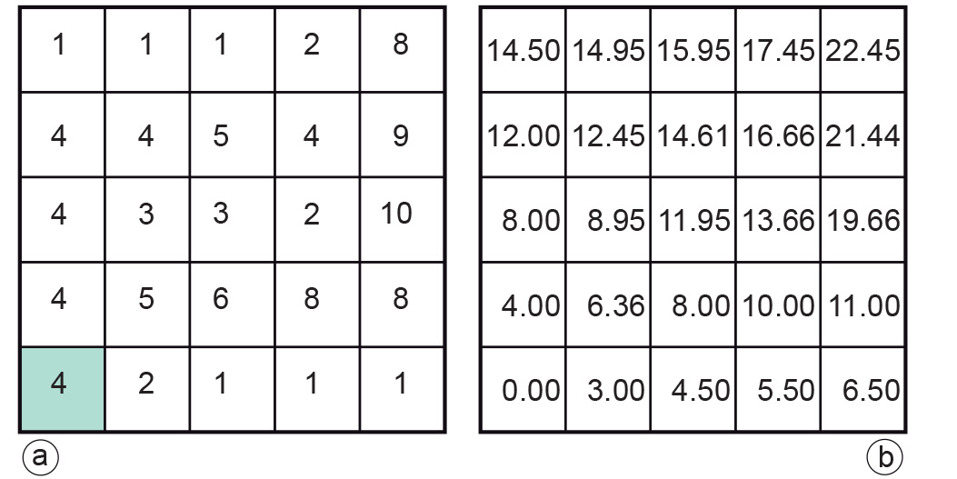
The value is found, for each cell, in the raster of Figure b.

For instance, there are three paths from the green source location to its northeast neighbour cell (with local resistance 5). We can define them as path 1 (N–E), path 2 (E–N) and path 3 (NE), using compass directions to define the path from the green cell. For path 1, the total resistance is computed as:

Path 2, in similar style, gives us a total value of 6.5. For path 3, we find:

and, thus, it is obviously the minimal cost path.

The reader is asked to verify one or two other values of minimal cost paths that the GIS has produced for the output raster.