Raster Overlay
Introduction
Vector overlay operators are useful but geometrically complicated, and this sometimes results in poor operator performance. Raster overlays do not suffer from this disadvantage, as most of them perform their computations cell by cell, and thus they are fast. GISs that support raster processing - as most do - usually have a language to express operations on rasters. These languages are generally referred to as map algebra or, sometimes, raster calculus. They allow a GIS to compute new rasters from existing ones, using a range of functions and operators. Unfortunately, not all implementations of map algebra offer the same functionality. The discussion below is to a large extent based on general terminology; it attempts to illustrate the key operations using a logical, structured language. Again, the syntax often varies among different GIS software packages.
Explanation
When producing a new raster we must provide a name for it, and define how it is to be computed. This is done in an assignment statement of the following format:
Output raster name := Map algebra expression.
The expression on the right is evaluated by the GIS, and the raster in which it results is then stored under the name on the left. The expression may contain references to existing rasters, operators and functions; the format is made clear in each case. The raster names and constants that are used in the expression are called its operands. When the expression is evaluated, the GIS will perform the calculation on a pixel-by-pixel basis, starting from the first pixel in the first row and continuing through to the last pixel in the last row. In map algebra, there is a wide range of operators and functions available.
Arithmetic operators
Various arithmetic operators are supported. The standard ones are multiplication (×), division (/), subtraction (-) and addition (+). Obviously, these arithmetic operators should only be used on appropriate data values, and, for instance, not on classification values. Other arithmetic operators may include modulo division (MOD) and integer division (DIV). Modulo division returns the remainder of division: for instance, 10 MOD 3 will return 1 as 10 - 3 × 3 = 1. Similarly, 10 DIV 3 will return 3.
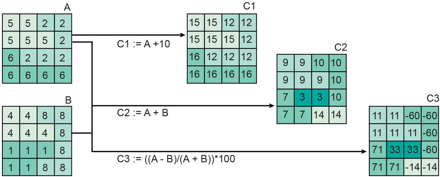
Other operators are goniometric: sine (sin), cosine (cos), tangent (tan); and their inverse functions asin, acos, and atan, which return radian angles as real values. Some simple map algebra assignments are illustrated in Figure 1 above. The assignment
C1 := A + 10
will add a constant factor of 10 to all cell values of raster A and store the result as output raster C1. The assignment
C2 := A + B
will add the values of A and B cell by cell, and store the result as raster C2. Finally, the assignment
C3 := (A - B) ∕ (A + B) × 100
will create output raster C3, as the result of the subtraction (cell by cell, as usual) of B cell values from A cell values, divided by their sum. The result is multiplied by 100. This expression, when carried out on AVHRR channel 1 (red) and AVHRR channel 2 (near infrared) of NOAA satellite imagery, is known as the NDVI (Normalized Difference Vegetation Index). It has proven to be a good indicator of the presence of green vegetation.
Comparison and logical operators
Map algebra also allows the comparison of rasters cell by cell. To this end, we may use the standard comparison operators (<, ⇐, =, >=, > and <>).

A simple raster comparison assignment is
C := A <> B.
It will store truth values—either true or false—in the output raster C. A cell value in C will be true if the cell’s value in A differs from that cell’s value in B. It will be false if they are the same. Logical connectives are also supported in many raster calculi. We have already seen the connectives of AND , OR and NOT in raster overlay operators. Another connective that is commonly offered in map algebra is exclusive OR (XOR). The expression a XOR b is true only if either a or b is true, but not both.

Examples of the use of these comparison operators and connectives are provided in Figure 2 and Figure 3. The latter figure provides various raster computations in searches for forests at specific elevations. In the figure, raster D1 indicates forest below 500 m, D2 indicates areas below 500 m or that are forests, raster D3 areas that are either forest or below 500 m (but not at the same time), and raster D4 indicates forests above 500 m.
Conditional expressions
The comparison and logical operators produce rasters with the truth values true and false. In practice, we often need a conditional expression together with them that allows us to test whether a condition is fulfilled. The general format is:
Output raster := CON(condition, then expression, else expression).
Here, condition stands for the condition tested, then the expression is evaluated if condition holds, and else the expression is evaluated if it does not hold. This means that an expression such as CON(A = “forest”, 10, 0) will evaluate to 10 for each cell in the output raster where the same cell in A is classified as forest. For each cell where this is not true, the else expression is evaluated, resulting in 0. Another example is provided in the Figure 4, showing that values for the then expression and the else expression can be some integer (possibly derived from another calculation) or values derived from other rasters. In this example, the output raster C1 is assigned the values of input raster B wherever the cells of input raster A contain forest. The cells in output raster C2 are assigned 10 wherever the elevation (B) is equal to 7 and the ground cover (A) is forest.

Overlays using a decision table
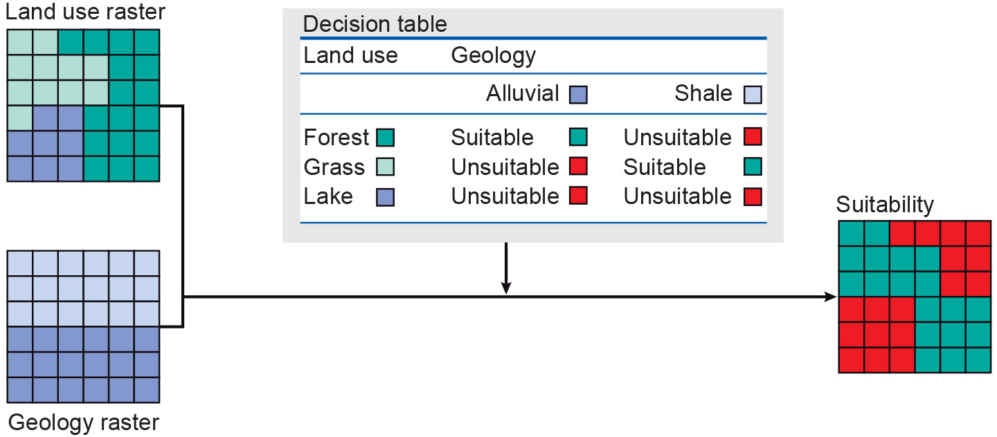
Conditional expressions are powerful tools in cases where multiple criteria must be taken into account. A small example may illustrate this. Consider a suitability study in which a land use classification and a geological classification must be used. The respective rasters are shown on the left-hand side of the Figure 5 below. Domain expertise dictates that some combinations of land use and geology result in suitable areas, whereas other combinations do not. In our example, forests on alluvial terrain and grassland on shale are considered suitable combinations, while any others are not.
We could produce the output raster of the Figure with a map algebra expression, such as
Suitability := CON((Landuse = “Forest” AND Geology = “Alluvial”)
OR (Landuse = “Grass” AND Geology = “Shale”),
“Suitable”, “Unsuitable”)
and consider ourselves lucky that there are only two “suitable” cases. In practice, many more cases must usually be covered and, then, writing up a complex CON expression is not an easy task.
To this end, some GISs accommodate setting up a separate decision table that will guide the raster overlay process. This extra table carries domain expertise and dictates which combinations of input raster-cell values will produce which output raster-cell value. This gives us a raster overlay operator using a decision table, as illustrated in the Figure 5. The GIS will have supporting functions to generate the additional table from the input rasters and to enter appropriate values in the table.
Learning outcomes
-
11 - Spatial analysis: classes of functions
Classify and explain spatial analysis functions (measurements, classification, overlay, neighbourhood and connectivity) in a raster and vector environment (level 1 and 2).
Prior knowledge
Outgoing relations
- Raster Overlay is a kind of Overlay Analysis
- Raster Overlay is used by Tessellation