14 - Data quality: data handling
Identify the impact of Geo-information handling on data quality (level 1).
Concepts
-
Data Quality
With the advent of satellite remote sensing,
GPS and GIS technology, and the increasing availability of digital spatial data, resource managers and others who formerly relied on the surveying and mapping profession to supply high quality map products are now in a position to produce maps themselves. At the same time,GIS s are being increasingly used for decision-support applications, with increasing reliance on secondary data sourced through data providers or via the internet, from geo-webservices. The consequences of using low-quality data when making important decisions are potentially grave. There is also a danger that uninformedGIS users will introduce errors by incorrectly applying geometric and other transformations to the spatial data held in their database.We discuss positional, temporal and attribute accuracy, lineage, completeness, and logical consistency.
-
Data checks and repairs
Data checks and repairs refers to the step when acquired data sets must be checked for quality in terms of the accuracy, consistency and completeness. Often, errors can be identified automatically, after which manual editing methods can be used to correct the errors. Alternatively, some software may identify and automatically correct certain types of errors. The geometric, topological, and attribute components of spatial data can be distinguished.

Figure 1: Clean-up operations for vector data. “Clean-up” operations are often performed in a standard sequence. For example, crossing lines are split before dangling lines are erased, and nodes are created at intersections before polygons are generated (Figure 1).
With polygon data, one usually starts with many polylines (in an unwieldy format known as spaghetti data) that are combined and cleaned in the first step (Figure 2a-b). This results in fewer polylines with nodes being created at intersections. Then, polygons can be identified (Figure 2c). Sometimes, polylines that should connect to form closed boundaries do not, and must, therefore, be connected either manually or automatically. In a final step, the elementary topology of the polygons can be derived (Figure 2d).
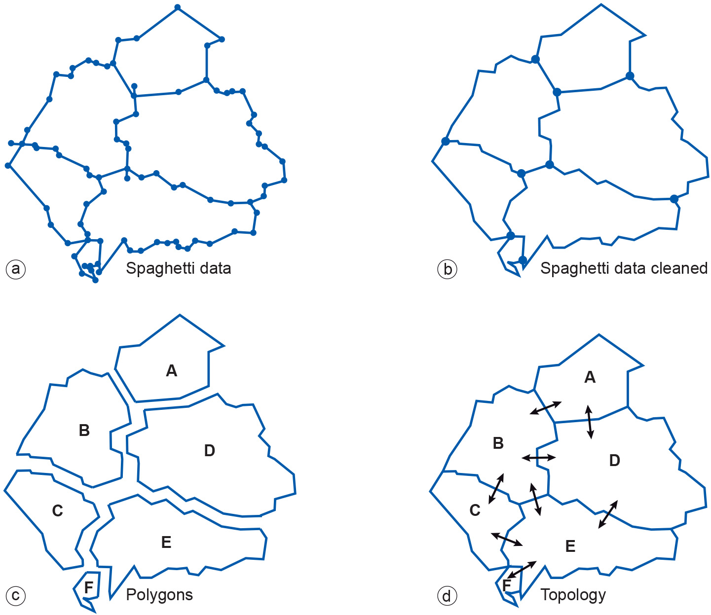
Figure 2: Successive clean-up operations for vector data, turning spaghetti data into topological structure. -
Data preparation
Spatial data preparation aims to make acquired spatial data fit for use. Images may require enhancements and corrections of the classification scheme of the data. Vector data also may require editing, such as the trimming of line overshoots at intersections, deleting duplicate lines, closing gaps in lines, and generating polygons. Data may require conversion to either vector or raster formats to match other data sets that will be used in analyses. Additionally, the data preparation process includes associating attribute data with the spatial features through either manual input or reading digital attribute files into the
GIS /DBMS .The intended use of the acquired spatial data may require a less-detailed subset of the original data set, as only some of the features are relevant for subsequent analysis or subsequent map production. In these cases, data and/or cartographic generalization can be performed on the original data set.
-
Associating attribute
Attributes may be automatically associated with features that have unique identifiers (Figure below). In the case of vector data, attributes are assigned directly to the features, while in a raster the attributes are assigned to all cells that represent a feature.

Figure: Attributes are associated with features that have unique identifiers. It follows that, depending on the data type, assessment of attribute accuracy may range from a simple check on the labelling of features - for example, is a road classified as a metalled road actually surfaced or not? - to complex statistical procedures for assessing the accuracy of numerical data, such as the percentage of pollutants present in a soil.
-
Rasterization
Rasterization, to convert vector data sets to raster data, involves assigning point, line and polygon attribute values to raster cells that overlap with the respective point, line or polygon. To avoid information loss, the raster resolution should be carefully chosen on the basis of the geometric resolution. A cell size that is too large may result in cells that cover parts of multiple vector features, and then ambiguity arises as to what value to assign to the cell. If, on the other hand, the cell size is too small, the file size of the raster may increase significantly.
Rasterization itself could be seen as a “backwards step”: firstly, raster boundaries are only an approximation of the objects’ original boundary. Secondly, the original “objects” can no longer be treated as such, as they have lost their topological properties. Rasterization is often done because it facilitates easier combination with other data sources that are also in raster formats, and/or because there are several analytical techniques that are easier to perform on raster data. An alternative to rasterization is to not perform it during the data preparation phase, but to use GIS rasterization functions “on the fly”, i.e. when the computations call for it. This allows the vector data to be kept and raster data to be generated from them when needed. Obviously, the issue of performance trade-offs must be looked into.
-
Topology generation
In Data checks and repairs we discussed the derivation of elementary polygon topology starting from uncleaned polylines. However, more topological relations may sometimes be needed, as for instance in networks where questions of line connectivity, flow direction and which lines have overpasses and underpasses may need to be addressed. For polygons, questions that may arise involve polygon inclusion: is a polygon inside another one, or is the outer polygon simply around the inner polygon?
In addition to supporting a variety of analytical operations, topology can aid in data editing and in ensuring data quality. For example, adjacent polygons such as parcels have shared edges; they do not overlap, nor do they have gaps. Typically, topology rules are first defined (e.g. “there should be no gaps or overlap between polygons”), after which validation of the rules takes place. The topology errors can be identified automatically, to be followed by manual editing methods to correct the errors.
An alternative to storing topology together with features in the spatial database is to create topology on the fly, i.e. when the computations call for it. The created topology is temporary, only lasting for the duration of the editing session or analysis operation.
-
Combining data from multiple sources
A GIS project usually involves multiple data sets, so this step addresses the issue of how these multiple sets relate to each other. The data sets may be of the same area but differ in accuracy, or they may be of adjacent areas, having been merged into a single data set, or the data sets may be of the same or adjacent areas but are referenced in different coordinate systems.
-
Accuracy differences
Differences in accuracy involve issues relating to positional error, attribute accuracy and temporal accuracy and are clearly relevant in any combination of data sets, which may themselves have varying levels of accuracy.
-
Differences in coordinate systems
It may be the case that data layers that are to be combined or merged in some way are referenced in different coordinate systems, or are based upon different datums. As a result, data may need a coordinate transformation, or both a coordinate transformation and datum transformation. It may also be the case that data have been digitized from an existing map or data layer. In this case, geometric transformations help to transform device coordinates (coordinates from digitizing tablets or screen coordinates) into world coordinates (geographic coordinates, metres, etc.).
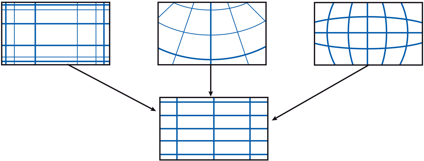
Figure: The integration of data sets into one common coordinate system. -
Error propagation
The acquisition of high quality base data still does not guarantee that the results of further, complex processing can be treated with certainty. As the number of processing steps increases, it becomes more difficult to predict the behaviour of such error propagation. These various errors may affect the outcome of spatial data manipulations. In addition, further errors may be introduced during the various processing steps.
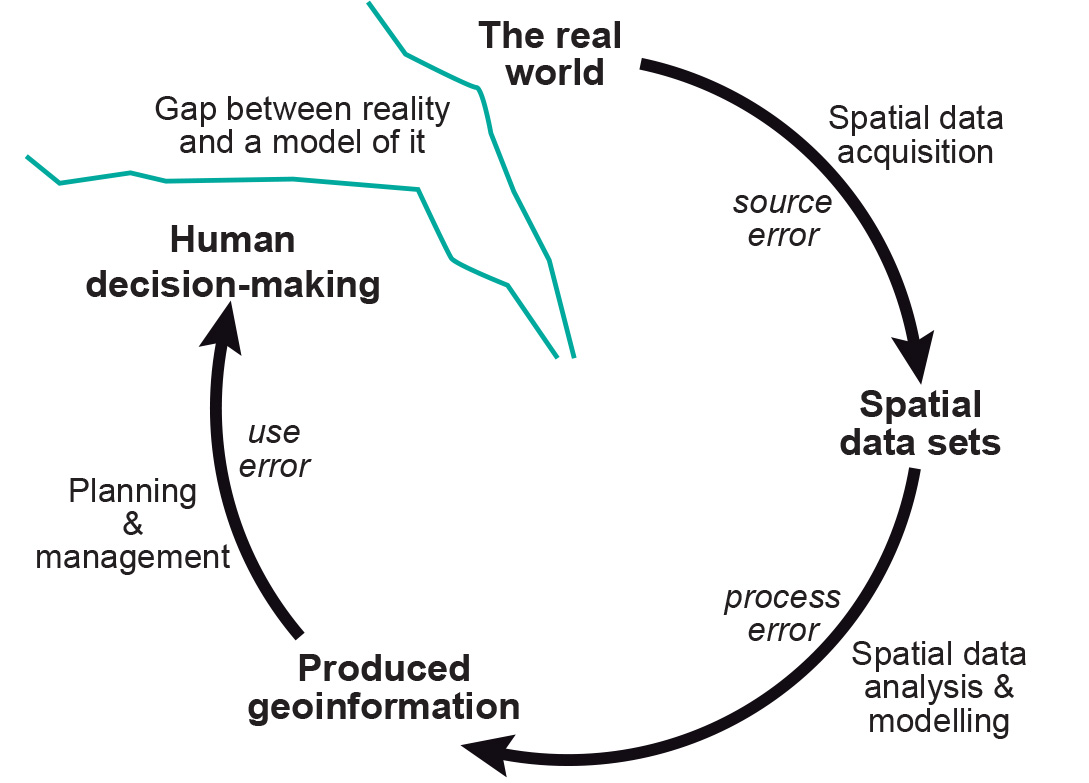
Figure: Error propagation in spatial data handling.