Error propagation

The acquisition of high quality base data still does not guarantee that the results of further, complex processing can be treated with certainty. As the number of processing steps increases, it becomes more difficult to predict the behaviour of such error propagation. These various errors may affect the outcome of spatial data manipulations. In addition, further errors may be introduced during the various processing steps.

Quantifying error propagation

Chrisman (1989) noted that:

We will never be able to capture and represent everything that happens in the real world perfectly in a GIS. Hence there is much to recommend the use of testing procedures for assessing accuracy. Various perspectives, motives and approaches for dealing with uncertainty have given rise to a wide range of conceptual models and indices for the description and measurement of error in spatial data. All these approaches have their origins in academic research and have solid theoretical foundations in mathematics and statistics. Here we identify two main approaches for assessing the nature and amount of error propagation:

1. testing the accuracy of each state by measurement against the real world; and

2. error propagation modelling, either analytically or by means of simulation techniques.

Common Sources of Error in GIS

This table lists some common sources of error that may be introduced into GIS analyses. Note that these originate in a wide range of sources and include various common tasks relating to both data preparation and data analysis. It is the combination of different errors that are generated at each stage of preparation and analysis that may result in several errors and uncertainties in the final outputs.

Error propagation modelling

Error propagation can be modelled mathematically, although these models are very complex and only valid for certain types of data(e.g. numerical attributes). Rather than explicitly modelling error propagation, it is often more practical to test the results of each step in the process against some independently measured reference data.

It is important to distinguish models of error from models of error propagation in GISs. Modelling of error propagation has been defined by Veregin (1995) as:

In other words, we would like to know how errors in the source data behave under the manipulations that we subject them to in a GIS. If we are able to quantify the error in the source data as well as their behaviour under GIS manipulations, we have a means of judging the uncertainty of their results.

Initially, error propagation models described only the propagation of attribute error (Heuvelink, 1993; Veregin, 1995). More recent research has addressed the spatial aspects of error propagation and the development of models incorporating both attribute and location components. These topics are beyond the scope of this book and readers are referred to Arbia et al. (1998) and Kiiveri (1997) for more details.

One of the most commonly applied operations in GISs is analysis by overlaying two or more spatial data layers. Each of these layers will contain errors, due to both inherent inaccuracies in the source data and errors arising from some form of computer processing - for instance, rasterization. During the process of spatial overlaying, errors in the individual data layers contribute to the final error of the output. The amount of error in the output depends on the type of overlay operation applied and on the amount of error in the individual layers. For example, errors in the results of an overlay using the logical operator AND are not the same as those created using the OR operator.

Consider another example. A land use planning agency is faced with the problem of identifying areas of agricultural land that are highly susceptible to erosion. Such areas occur on steep slopes in areas of high rainfall. The spatial data used in a GIS to obtain this information might include:

• a land use map produced five years previously from 1:25,000 scale aerial photographs;

• a DEM produced by interpolating contours from a 1:50,000 scale topographic map; and

• annual rainfall statistics collected with two rainfall gauges.

The reader is invited to assess what sort of errors are likely to occur in this analysis.

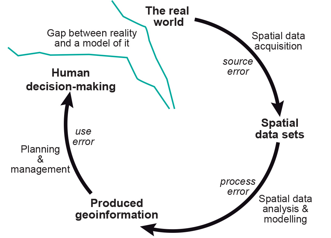
Referring back to the Figure above, the reader is also encouraged to reflect on errors introduced in the components of the application models, specifically, the methodological aspects of representing geographic phenomena. What might be the consequences of using a random function in an urban transportation model (when, in fact, travel behaviour is not purely random)?