3 - Spatial data modelling: topology

Concepts

• Topological data model

  The boundary model is an improved representation that deals with the disadvantages of the naive polygon which is described in polygons. It stores parts of a polygon’s boundary as non-looping arcs and indicates which polygon is on the left and which is on the right of each arc. A simple example of the boundary model can be seen below. It illustrates which additional information is stored about spatial relationships between lines and polygons. Obviously, real coordinates for nodes (and vertices) will also be stored in another table. The boundary model is also called the topological data model as it captures some topological information, such as polygon neighbourhood, for example. You can read more about topological information in Topology. Observe that it is a matter of a simple query to find all the polygons that are the neighbour of a given polygon, unlike the case above.

• Topological Consistency

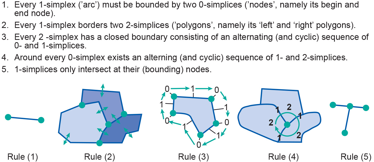
  Rules of how simplices and simplicial complexes can be embedded in 2D and 3D space are quite different. Such a set of rules defines the topological consistency of that space. It can be proven that if the rules presented and illustrated in the Figure below are satisfied for all features in 2D space, then the features define a topologically consistent configuration in 2D space.

  

  This also plays an important rule during Data Checks and Repairs during Data Preparation.

  Topological Consistency in 3D

  Our discussion of vector representations and spatial topology has so far focused on objects in 2D space. The history of spatial data handling is almost purely 2D, and this is remains the case for the majority of present-day GIS applications. Many application domains make use of elevational data, but these are usually accommodated for by what are known as 2.5D data structures. These 2.5D data structures are similar to the 2D data structures just discussed, using points, lines and areas. They also apply the rules of two-dimensional topology, as illustrated in the Figure above. This means that different lines cannot cross without intersecting nodes and that different areas cannot overlap. There is, however, one important aspect in which 2.5D data do differ from standard 2D data and that is in their association of an additional z-value with each 0-simplex (‘node’). Thus, nodes also have an elevation value associated with them. Essentially, this allows the GIS user to represent 1- and 2-simplices that are non-horizontal, so that a piece-wise planar, “wrinkled surface” can be constructed as well, much like a TIN. One cannot have two different nodes with identical x and y coordinates but different z values. Such nodes would constitute a perfectly vertical feature, which is not allowed. Consequently, true solids cannot be represented in a 2.5D GIS.

• Topological relationship

  We can use the topological properties of interiors and boundaries to define relationships between spatial features. Since the properties of interiors and boundaries do not change under topological mapping, we can investigate their possible relations between spatial features. We can define the interior of a region, R, as the largest set of points of R for which we can construct a disc-like environment around it (no matter how small) that also falls completely inside R. The boundary of R is the set of those points belonging to R that do not belong to the interior of R, i.e. one cannot construct a disc-like environment around such points that still belongs to R completely.

• Topology

  Topology refers to the spatial relationships between geographic elements in a data set that do not change under a continuous transformation. This is defined by topological relationships.