Map type
Introduction
Traditionally, maps have been divided into two sorts: topographic maps and thematic maps.
A topographic map visualizes, limited by its scale, the Earth’s surface as accurately as possible. This may include infrastructure (e.g. railways and roads), land use (e.g. vegetation and built-up areas), relief, hydrology, geographic names and a reference grid.
Thematic maps represent the distribution of particular themes. One can distinguish between socio-economic themes and physical themes.
Explanation
Thematic maps also contain some information found in the topographic maps. The amount of topographic information required depends on the map theme. In general, a physical map will need more topographic data than most socio-economic maps, which normally only need administrative boundaries. The map of drainage areas should have had rivers and canals added, while the inclusion of relief would also have made sense. Today’s digital environment has diminished the distinction between topographic and thematic maps. Often, both topographic and thematic maps are stored in a database as separate data layers. Each layer contains data on a particular topic and the user is able to switch layers on or off at will.
The design of topographic maps is mostly based on conventions, some of which date back several centuries. Take, for example the following colour conventions: water in blue, forests in green, major roads in red, and urban areas in black. The design of thematic maps, however, should be based on a set of cartographic rules, also called cartographic grammar.
Suppose that one wants to quantify land use changes in a certain area between 1990 and the current year. Two data sets (from 1990 and, say, 2008) can be combined with an Overlay Analysis. The result of such a spatial analysis could be a spatial data layer from which a map can be produced to show the differences. The parameters used during the operation are based on models developed by the application at hand. It is easy to imagine that maps can play a role during this process of working with a GIS, by showing intermediate and final results of the GIS operations. Clearly, maps are no longer the only final product, which they used to be.
Maps can further be distinguished according to the dimensions of spatial data that are graphically represented. GIS users also try to solve problems that deal with three-dimensional reality or with change processes. This results in a demand for other than just two-dimensional maps to represent geographic reality. Threedimensional and even four-dimensional (namely, including time) maps are then required. New visualization techniques for these demands have been developed.
Examples
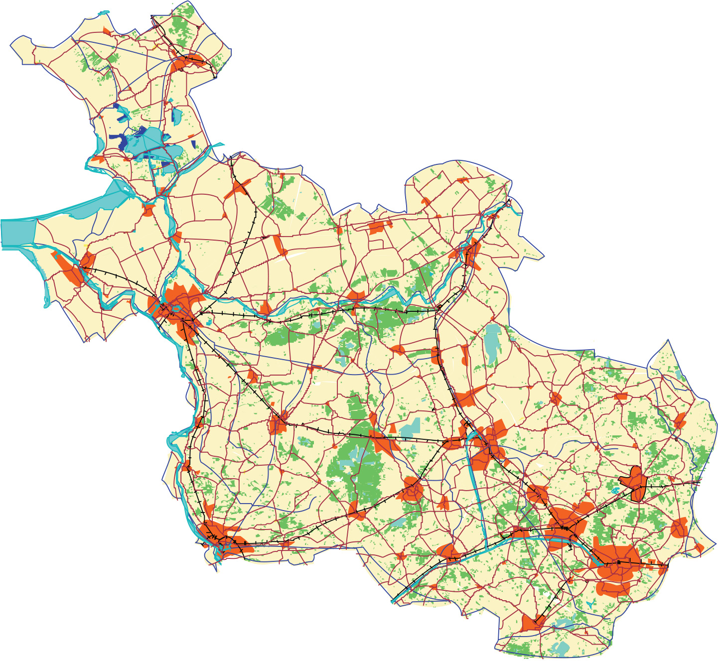
Figure 1 shows a small-scale topographic map (with text omitted) of Overijssel, the Dutch province in which Enschede is located.
Thematic maps can have socio-economic themes and physical themes. The map in Figure 2a, showing population density in Overijssel, is an example of the first and the map in Figure 2b, displaying the province’s drainage areas, is an example of the second.
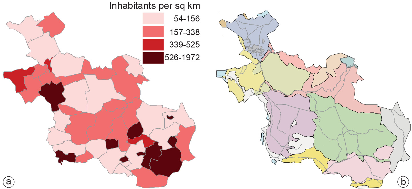
watershed areas of Overijssel.
As can be observed, both thematic maps also contain some information found in the topographic map (Figure 1), so as to provide a geographic reference to the theme represented.
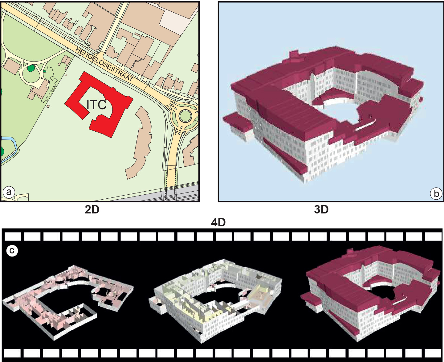
Figure 3 shows the dimensionality of geographic objects and their graphic representation. Part (a) shows a map of the ITC building and its surroundings, while part (b) provides a three-dimensional view of the building. Figure 3c shows the effect of change, at three moments in time during the construction of the building.
Outgoing relations
- Map type is a property of Map