RMSE

Positional accuracy is normally measured as a root mean square error (RMSE). The RMSE is similar to, but not to be confused with, the standard deviation of a statistical sample. 

The value of the RMSE is normally calculated from a set of check measurements (coordinate values from an independent source of higher accuracy for identical points). The differences at each point can be plotted as error vectors, as is done in the Figure 1 below for a single measurement. The error vector can be seen as having constituents in the x- and y- directions, which can be recombined by vector addition to give the error vector representing the locational error.

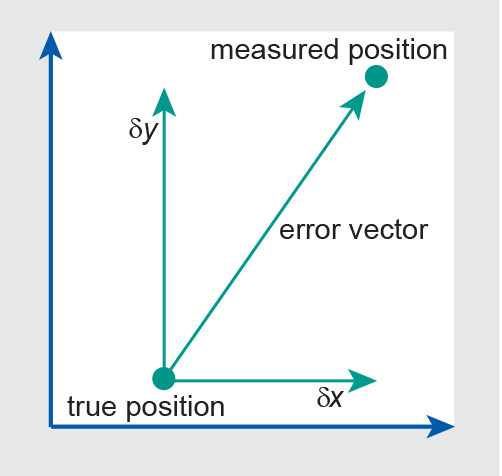
For each checkpoint, the error vector has components δx and δy. The observed errors should be checked for a systematic error component, which may indicate a (possibly repairable) lapse in the measurement method. Systematic error has occurred when ∑δx≠0 or ∑δy≠0.

The systematic error δx in x is then defined as the average deviation from the true value:

Analogously to the calculation of the variance and standard deviation of a statistical sample, the root mean square errors m_x and m_y of a series of coordinate measurements are calculated as the square root of the average squared deviations:

where δx² stands for δx ⋅ δx. The total RMSE is obtained with the formula

which, by the Pythagorean rule, is the length of the average (root squared) vector.

Accuracy tolerances

Many kinds of measurement can be naturally represented by a bell-shaped probability density function p, as depicted in Figure 2(a). This function is known as the normal (or Gaussian) distribution of a continuous, random variable, in the figure indicated as Y . It shape is determined by two parameters: μ, which is the mean expected value for Y , and σ, which is the standard deviation of Y . A small σ leads to a more attenuated bell-shaped function.

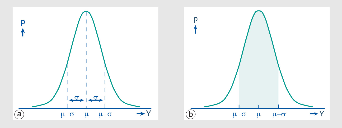
Any probability density function p has the characteristic that the area between its curve and the horizontal axis is equal to 1. Probabilities P can be inferred from p as the area under p’s curve. Figure 2(b), for instance, depicts P(μ-σ ≤ Y ≤ μ-σ), i.e. the probability that the value for Y is within distance σ from μ. In a normal distribution this specific probability for Y is always 0.6826.

The RMSE can be used to assess the probability that a particular set of measurements does not deviate too much from, i.e. is within a certain range of, the “true” value. In the case of coordinates, the probability density function is often considered to be that of a two-dimensional normally distributed variable (see Figure 3). The three standard probability values associated with this distribution are:

• 0.50 for a circle with a radius of 1.1774 m_x around the mean (known as the circular error probable, CEP);

• 0.6321 for a circle with a radius of 1.412 m_x around the mean (known as the root mean square error, RMSE);

• 0.90 for a circle with a radius of 2.146 m_x around the mean (known as the circular map accuracy standard, CMAS).

The RMSE provides an estimate of the spread of a series of measurements around their (assumed) “true” values. It is therefore commonly used to assess the quality of transformations such as the absolute orientation of photogrammetric models or the spatial referencing of satellite imagery. The RMSE also forms the basis of various statements for reporting and verifying compliance with defined map accuracy tolerances. An example is the American National Map Accuracy Standard, which states that:

“No more than 10% of well-defined points on maps of 1:20,000 scale or greater may be in error by more than 1/30 inch.”

Normally, compliance to this tolerance is based on at least 20 well-defined checkpoints. The Epsilon Band  is often used for confidence levels.