Reclassification
Introduction
Classification is a technique for purposely removing detail from an input data set in the hope of revealing important patterns (of spatial distribution). In the process, we produce an output data set, so that the input set can be left intact. This output set is produced by assigning a characteristic value to each element in the input set, which is usually a collection of spatial features that could be raster cells or points, lines or polygons. If the number of characteristic values in the output set is small in comparison to the size of the input set, we have classified the input set.
The input data set may, itself, have been the result of a classification. In such cases we refer to the output data set as a reclassification. For example, we may have a soil map that shows different soil type units and we would like to show the suitability of units for a specific crop. In this case, it is better to assign to the soil units an attribute of suitability for the crop. Since different soil types may have the same crop suitability, a classification may merge soil units of different type into the same category of crop suitability.
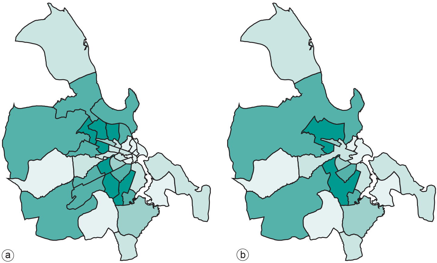
In classification of vector data, there are two possible results. In the first, the input features may become the output features in a new data layer, with an additional category assigned. In other words, nothing changes with respect to the spatial extents of the original features. Figure a of Examples illustrates this first type of output. A second type of output is obtained when adjacent features of the same category are merged into one bigger feature. Such a post-processing function is called spatial merging, aggregation or dissolving. An illustration of this second type is found in Figure b of Examples. Observe that this type of merging is only an option in vector data, as merging cells in an output raster on the basis of a classification makes little sense. Vector data classification can be performed on point sets, line sets or polygon sets; the optional merge phase only makes sense for lines and polygons.
Examples

The pattern that we are looking for may be the distribution of household income in a city. In that case, household income is called the classification parameter. If we know for each ward in the city the associated average income, we have many different values. Subsequently, we could define five different categories (or classes) of income: “low”, “below average”, “average”, “above average” and “high”, and provide value ranges for each category (see Table below). If these five categories are mapped using a sensible colour scheme, this may reveal interesting information. The Figure above illustrates how this has been done in two ways for Dar es Salaam.
| Household income range | New category value |
|---|---|
| 391–2474 | 1 |
| 2475–6030 | 2 |
| 6031–8164 | 3 |
| 8165–11587 | 4 |
| 11588–21036 | 5 |
Learning outcomes
-
11 - Spatial analysis: classes of functions
Classify and explain spatial analysis functions (measurements, classification, overlay, neighbourhood and connectivity) in a raster and vector environment (level 1 and 2).
Prior knowledge
Outgoing relations
- Reclassification is a kind of Analysis
- Reclassification is used by Tessellation
- Reclassification is used by Vector Representation
Incoming relations
- Automatic reclassification is a kind of Reclassification
- User controlled classification is a kind of Reclassification