Histogram
Introduction
A histogram shows the number of pixels having each value, i.e. the frequency distribution of the DNs. Histogram data can be represented either in tabular form or graphically.
The tabular representation usually shows five columns (see Table 1 in the Examples). From left to right these are:
-
DN: Digital Numbers, in the range 0–255
-
Npix: the number of pixels in the image with a particular DN (frequency)
-
Perc: frequency as a percentage of the total number of image pixels
-
CumNpix: cumulative number of pixels in the image with values less than or equal to a particular DN
-
CumPerc: cumulative frequency as a percentage of the total number of image pixel.
Graphically, more commonly, the histogram is displayed as a bar graph rather than as a line graph.
Examples
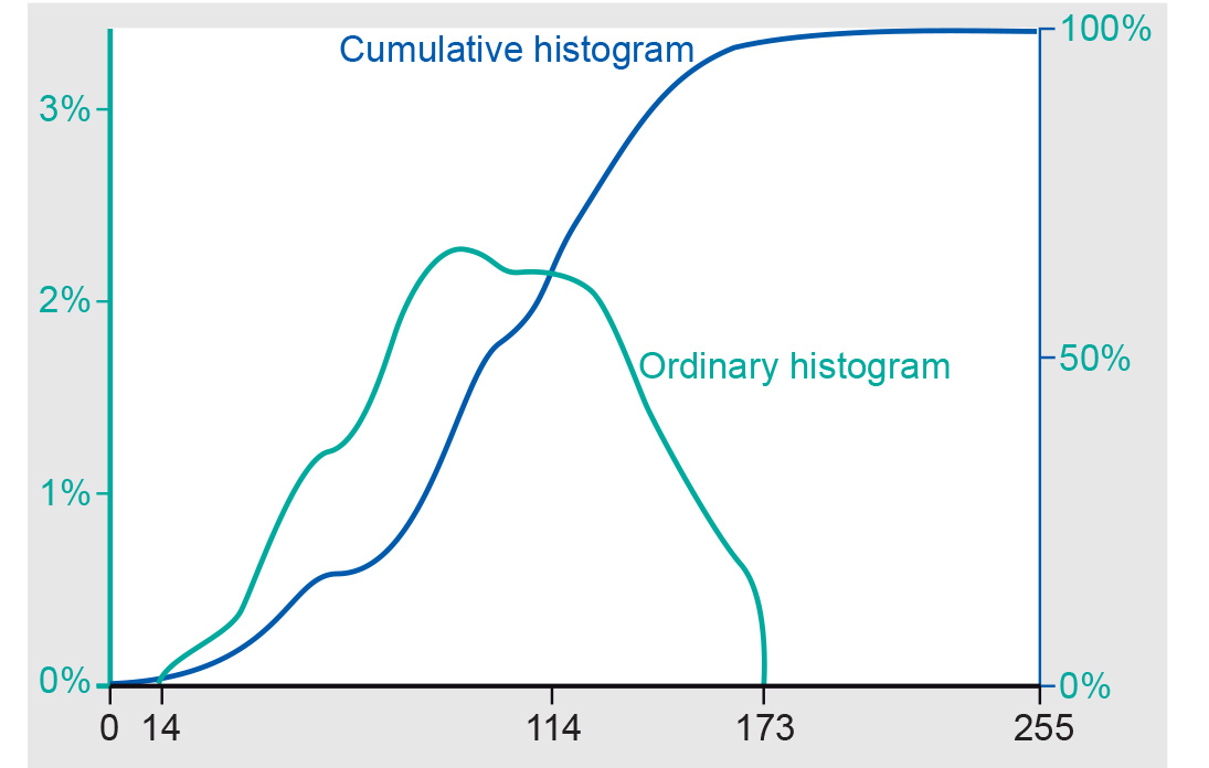
The Figure 1 shows a plot of the columns 3 and 5 of Table 1 against column 1. The graphical representation of column 5 can readily be used to find the ‘1% value’ and the ‘99% value’. The 1% value is the DN, below which only 1% of all the values are found. Similarly, there are only 1% of all the pixels of the image having a DN value larger than the 99% value. The 1% and 99% values are often used in histogram operations as cut-off values for display, thus classifying very small and very large DNs as noise outliers rather than signals.
| DN | Npix | Perc | CumNpix | CumPerc |
| 0 | 0 | 0.00 | 0 | 0.00 |
| 13 | 0 | 0.00 | 0 | 0.00 |
| 14 | 1 | 0.00 | 1 | 0.00 |
| 15 | 3 | 0.00 | 4 | 0.01 |
| 16 | 2 | 0.00 | 6 | 0.01 |
| 51 | 55 | 0.08 | 627 | 0.86 |
| 52 | 59 | 0.08 | 686 | 0.94 |
| 53 | 94 | 0.13 | 780 | 1.07 |
| 54 | 138 | 0.19 | 918 | 1.26 |
| 102 | 1392 | 1.90 | 25118 | 34.36 |
| 103 | 1719 | 2.35 | 26837 | 36.71 |
| 104 | 1162 | 1.59 | 27999 | 38.30 |
| 105 | 1332 | 1.82 | 29331 | 40.12 |
| 106 | 1491 | 2.04 | 30822 | 42.16 |
| 107 | 1685 | 2.31 | 32507 | 44.47 |
| 108 | 1399 | 1.91 | 33906 | 46.38 |
| 109 | 1199 | 1.64 | 35105 | 48.02 |
| 110 | 1488 | 2.04 | 36593 | 50.06 |
| 111 | 1460 | 2.00 | 38053 | 52.06 |
| 163 | 720 | 0.98 | 71461 | 97.76 |
| 164 | 597 | 0.82 | 72058 | 98.57 |
| 165 | 416 | 0.57 | 72474 | 99.14 |
| 166 | 274 | 0.37 | 72748 | 99.52 |
| 173 | 3 | 0.00 | 73100 | 100.00 |
| 174 | 0 | 0.00 | 73100 | 100.00 |
| 255 | 0 | 0.00 | 73100 | 100.00 |
A histogram can also be “summarized” by descriptive statistics: mean, standard deviation, minimum and maximum, as well as the 1% and 99% values (Table 2). The mean is the average of all the DNs of the image; note that it often does not coincide with the DN that appears most frequently. The standard deviation indicates the spread of DNs around the mean.
| Mean | StdDev | Min | Max | 1% value | 99% value |
| 113.79 | 27.84 | 14 | 173 | 53 | 165 |
Incoming relations
- Histogram operation is based on Histogram