Histogram operation
Introduction
Histogram operations aim at global contrast enhancement, also referred to as contrast enhancement, in order to increase the visual distinction between features. The radiometric properties of a digital image are revealed by its histogram, which describes the distribution of the pixel values of the image. By changing the histogram, we change the visual quality of the image.
Although contrast enhancement may be done for different purposes, ultimately, in all cases, we will only do so to improve the visual interpretability of an image. In fact, there are two main purposes for applying contrast enhancement. The first is for “temporary enhancement”, where we do not want to change the original data but only want to get a better image on the monitor so that we can carry out a specific interpretation task. Image display for geometric correction is an example of this. The second purpose is to generate new data that have a higher visual quality than the original data. This would be the case if an image is to be the output of our RS activities. Orthophoto production and image mapping are examples of such output.
Explanation
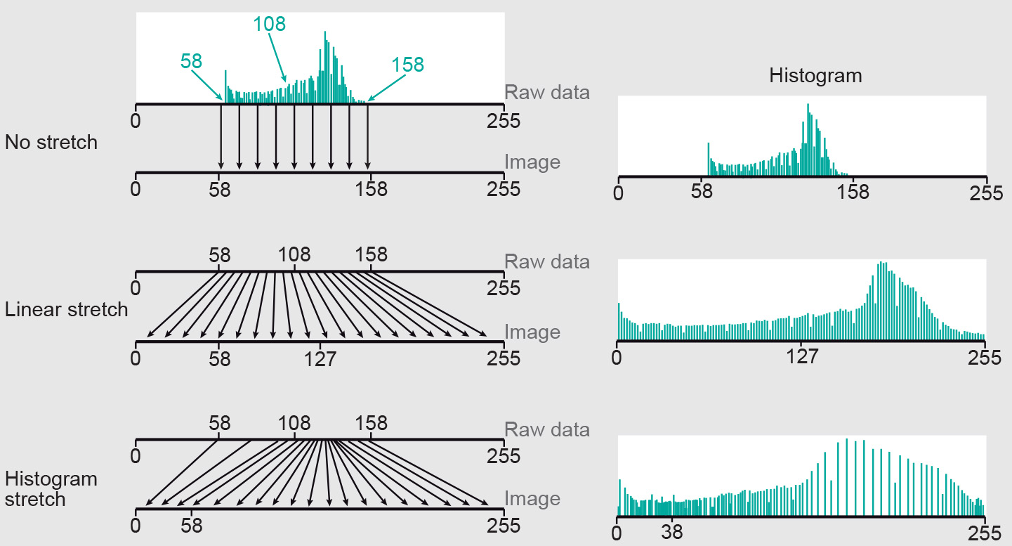
Two techniques of contrast enhancement will be described: linear contrast stretch and histogram equalization (occasionally also called histogram stretch). Both are “grey scale transformations”, which convert input DNs (of raw data) to new brightness values (for a more appealing image) by a user-defined “transfer function”.
Linear contrast stretch is a simple grey scale transformation in which the lowest input DN of interest becomes zero and the highest DN of interest becomes 255 (Figure 1). The monitor will display zero as black and 255 as white. In practice, we often use the 1% and 99% values as the lowest and highest input DNs. The functional relationship between the input DNs and output pixel values is linear, as shown in the example Figure 2a. The functions shown in the first row (a, d, g) of the example Figure 2 (in the background of the histogram of each input image) are called the transfer functions. Many image processing software packages allow users to graphically manipulate the transfer function so that they can obtain an image that appears to their liking. The actual transformation is usually based on a look-up table.
The transfer function to be used can be chosen in a number of ways. We can use linear grey-scale transformation to correct for haze and also for other purposes than contrast stretching, for instance to “invert an image” (convert a negative image to a positive one, or vice versa) or to produce a binary image (the simplest technique of image segmentation). Inverting an image is relevant, for example, after having scanned a negative of a photograph.
Linear stretch is a straight-forward method of contrast enhancement that gives fair results when the input image has a narrow histogram that has a distribution close to being uniform.
As the name suggests, histogram equalization aims at achieving a more uniform distribution in the histogram. Histogram equalization is a non-linear transformation; several image processing packages offer it as a default function. The idea can be generalized to achieve any desired target histogram.
It is important to note that contrast enhancement (by linear stretch or histogram equalization) merely amplifies small differences between DN values so that we can visually differentiate between features more easily. Contrast enhancement does not, however, increase the information content of the data and it does not consider a pixel neighbourhood. Histogram operations should be based on analysis of the shape and extent of the histogram of the raw data and understanding what is relevant for the intended interpretation. If this is not done, a decrease of information content could easily occur.
Examples
A narrow histogram (thus, a small standard deviation) represents an image of low contrast, because all the DNs are very similar and are initially mapped to only a few grey values. Notice the peak at the upper end in the figure below (DN larger than 247), while most of DNs are smaller than 110. The peak for the white pixels stems from the sky. All other pixels are dark greyish; this narrow part of the histogram characterizes the poor contrast of the image (a Maya monument in Mexico). Remote sensors commonly use detectors with a wide dynamic range, so that they can sense under a wide variety of different illumination and emission conditions. These differences, however, are not always present in one particular scene. In practice, therefore, we often obtain RS images that do not exploit the full range of DNs. A simple technique to achieve better visual quality is, then, to enhance the contrast by “grey scale transformation”, which yields a histogram stretched over the entire grey range of pixels on the computer monitor.
The histogram of our example image is asymmetric, with all DNs in a small range at the lower end, if the irrelevant sky pixels are not considered. Stretching this small range with high frequencies of occurrence (Figure 2d) at the expense of compressing the range with only few values (in our example, the range of high brightness) will make more detail visible in the dark parts of the original (Figure 2e).
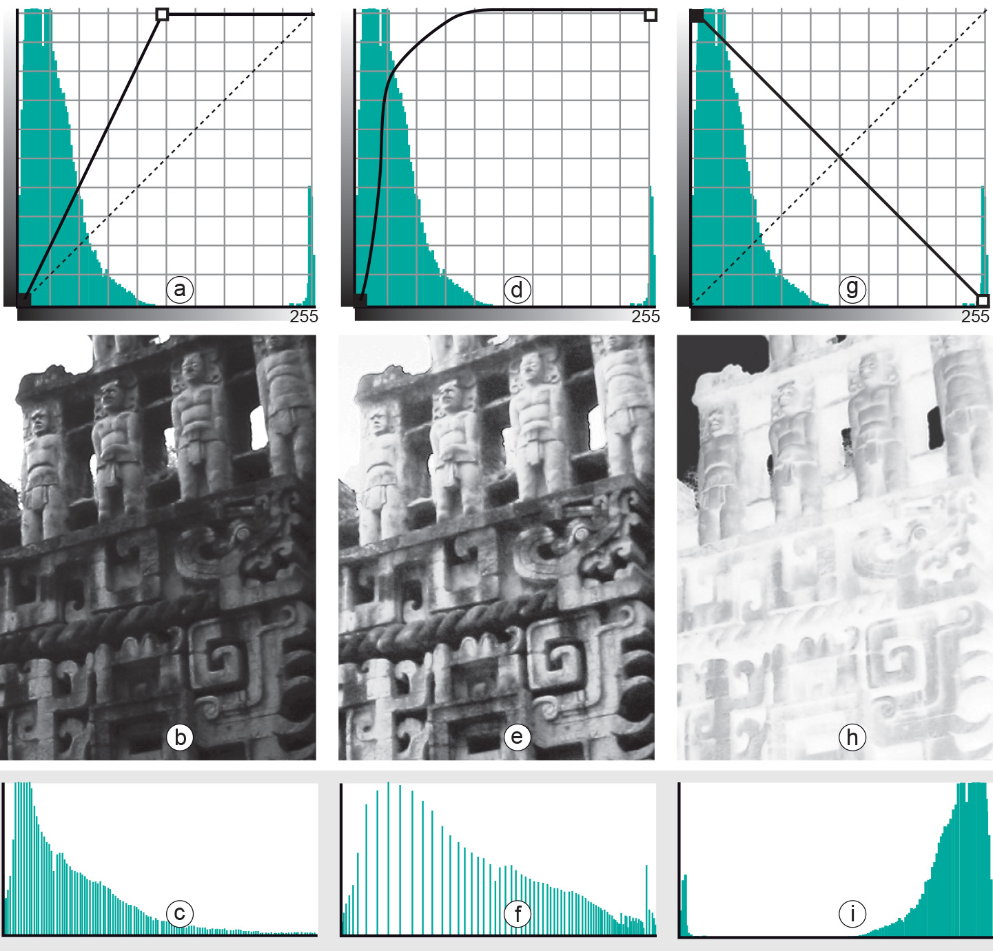
Histogram equalization allows to achieve a more uniform distribution in the histogram (Figure 2f).
Prior knowledge
Outgoing relations
- Histogram operation is a kind of Image enhancement
- Histogram operation is based on Histogram
Incoming relations
- Global contrast enhancement is same as Histogram operation