Pixel based classifcation
Introduction
Pixel-based image classification is a powerful technique to derive thematic classes from multi-band images. However, it has certain limitations that users should be aware of. The most important constraints of pixel-based image classification are that it results in (i) spectral classes, and that (ii) each pixel is assigned to one class only.
Explanation
Spectral classes are those that are directly linked to the spectral bands used in the classification. In turn, these are linked to surface characteristics. In that respect, one can say that spectral classes correspond to land cover classes. In the classification process a spectral class may be represented by several training classes. Among other things, this is due to the variability within a spectral class. Consider, for example, a class such as “grass”: there are different types of grass, each of which has different spectral characteristics. Furthermore, the same type of grass may have different spectral characteristics when considered over larger areas, owing to, for example, different soils and climatic conditions.
A related issue is that sometimes one is interested in land use classes rather than land cover classes. Sometimes, a land use class may comprise several land cover classes. Table 1 gives some examples of links between spectral land cover and land use classes. Note that between two columns there can be 1-to-1, 1-to-n, and n-to-1 relationships. The 1-to-n relationships are a serious problem and can only be solved by adding data and/or knowledge to the classification procedure. The data added can be other remote sensing images (other bands, other moments) or existing geospatial data, such as topographic maps, historical land inventories, road maps, and so on. Usually this is done in combination with adding expert knowledge to the process. An example would be using historical land cover data and defining the probability of certain land cover changes. Another example would be to use elevation, slope and aspect information. This will prove especially useful in mountainous regions, where elevation differences play an important role in variations of surface-cover types.
Add Table: Spectral classes distinguished during classification can be aggregated to land cover classes. 1-to-n and n-to-1 relationships can exist between land cover and land use classes.
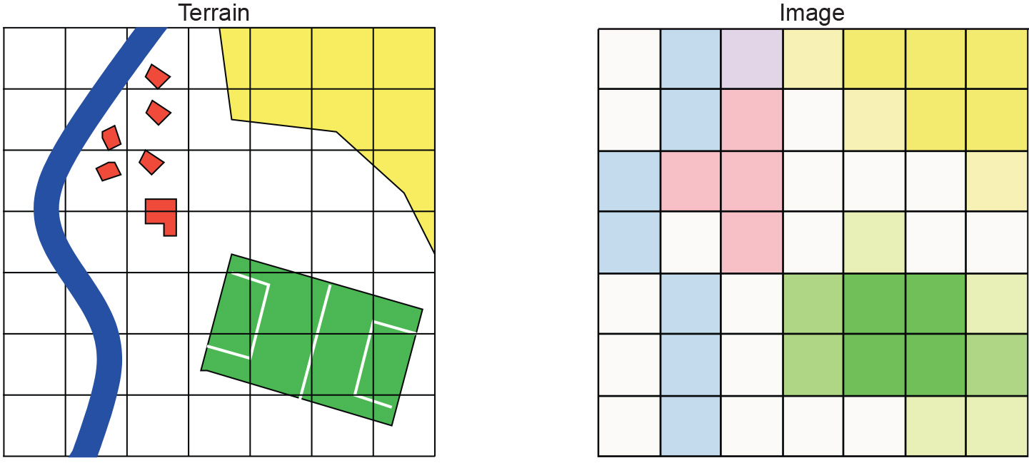
The other main problem and limitation of pixel-based image classification is that each pixel is only assigned to one class. This is not a problem when dealing with relatively small ground resolution cells. However, when dealing with relatively large GRCs, more land cover classes are likely to occur within a cell. As a result, the value of the pixel is an average of the reflectance of the land cover present within the GRC. In a standard classification, these contributions cannot be traced back and the pixel will be assigned to one of either classes or perhaps even to another class. This phenomenon is usually referred to as the mixed pixel, or mixel (Figure 1). This problem of mixed pixels is inherent to image classification: assigning a pixel to one thematic class. The solution to this is to use a different approach, for example, by assigning the pixel to more than one class. This brief introduction into the problem of mixed pixels also highlights the importance of using data with the appropriate spatial resolution.
We have seen that the choice of classification approach depends on the data available, but also on the knowledge we have about the area under investigation. Without knowledge of the land cover classes present, unsupervised classification can only give an overview of the variety of classes in an image. If knowledge is available, from field work or other sources, supervised classification may be superior. However, both methods only make use of spectral information, which becomes increasingly problematic for higher spatial resolutions. For example, a building that is made up of different materials leads to pixels with highly variable spectral characteristics, and thus a situation for which training of pixels is of little help. Similarly, a field may contain healthy vegetation pixels as well as some of bare soil.
Outgoing relations
- Pixel based classifcation is a kind of Digital Image Classification
Incoming relations
- Supervised Image Classfication Algorithm is a kind of Pixel based classifcation
- Unsupervised Image Classification Algorithm is a kind of Pixel based classifcation