Geocoding

Geocoding is georeferencing with subsequent resampling of the image raster. This means that a new image raster is defined along the x- and y-axes of the selected map projection.

Georeferencing explained that two-dimensional coordinate systems, e.g. an image system and a map system, can be related using geometric transformations. This georeferencing approach is useful in many situations. However, in some situations a geocoding approach, in which the row–column structure of the image is also transformed, is required. Geocoding is required when different images need to be combined or when the images are used in a GIS environment that requires all data to be stored in the same map projection. Distinguishing georeferencing and geocoding is conceptually useful, but to the casual software user it is often not apparent whether only georeferencing has been applied in certain image manipulations or also geocoding.

The effect of geocoding is illustrated in the Figure below along with a georeferencing example.  

The geocoding process comprises three main steps: (1) selection of a new grid spacing; (2) projection (using the transformation parameters) of each new raster element onto the original image; and (3) determination and storage of a DN for the new pixel.

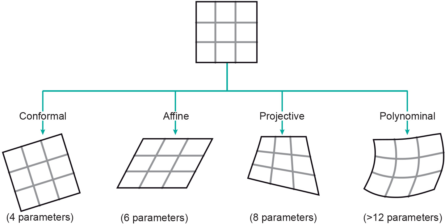
Figure 1 shows four transformation types that are frequently used in RS. The types shown increase from left to right in complexity and number of parameters required. In a conformal transformation, the image shape, including right angles, are retained. Therefore, only four parameters are needed to describe a shift along the x- and y-axes, a scale change, and the rotation. However, if you want to geocode an image to make it fit with another image or map, a higher-order transformation may be required, such as a projective or polynomial transformation.

Most of the projected raster elements of the new image will not match precisely with raster elements in the original image, as Figure 2 illustrates. Since raster data are stored in a regular row–column pattern, we need to calculate DNs for the pixel pattern of the corrected image intended. This calculation is performed by interpolation. This is called resampling of the original image.

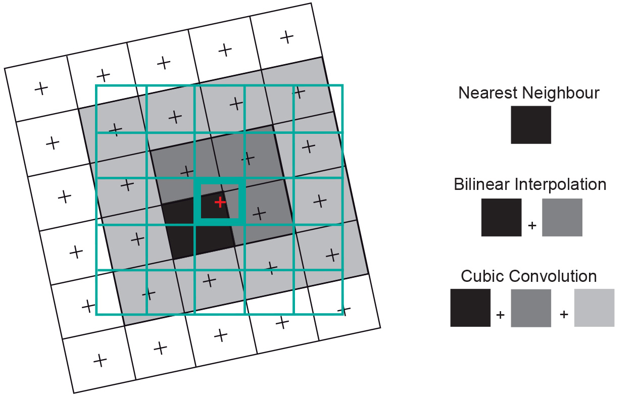
For resampling, we usually use very simple interpolation methods, the main ones being nearest neighbour, bilinear, and bicubic interpolation (Figure 2). Consider the green grid to be the output image to be created. To determine the value of the centre pixel (bold), in nearest neighbour interpolation the value of the nearest original pixel is assigned, i.e. the value of the black pixel in this example. Note that the respective pixel centres, marked by small crosses, are always used for this process. In bilinear interpolation, a linear weighted average is calculated for the four nearest pixels in the original image (dark grey and black pixels). In bicubic interpolation a cubic weighted average of the values of 16 surrounding pixels (the black and all grey pixels) is calculated. Note that some software uses the terms “bilinear convolution” and “cubic convolution” instead of the terms introduced above.

The choice of the resampling algorithm depends, among other things, on the ratio between input and output pixel size and the intended use of the resampled image. Nearest neighbour resampling can lead to the edges of features being offset in a step-like pattern. However, since the value of the original cell is assigned to a new cell without being changed, all spectral information is retained, which means that the resampled image is still useful in applications such as digital image classification. The spatial information, on the other hand, may be altered in this process, since some original pixels may be omitted from the output image, or appear twice. Bilinear and bicubic interpolation reduce this effect and lead to smoother images. However, because the values of a number of pixels are averaged, radiometric information is changed (Figure 3).