System Modelling

Application models (system models) varying in nature. GIS applications for famine-relief programmes, for instance, are different from earthquake-risk assessment applications, though both use GISs to derive a solution. Many kinds of application models exist and they can usually be classified in various ways. Here we identify five ways of classifying the characteristics of GIS-based application models (compare with the model of Randers in Model Characteristic):

• the purpose of the model;

• the methodology underlying the model;

• the scale at which the model works;

• its dimensionality, i.e. whether the model includes spatial, temporal or spatial and temporal dimensions;

• its implementation logic, i.e. the extent to which the model uses existing knowledge about the implementation context.

These classifications express different ways for classifying model characteristics. Any application model has characteristics that can be described according to the above categories. Each of these is briefly discussed here.

Purpose of the model

The purpose of a model refers to whether the model is descriptive, prescriptive or predictive in nature. Descriptive models attempt to answer the “what is” question. Prescriptive models answer the “what should be” question by determining the best solution from a given set of conditions. Models for planning and site selection are prescriptive in that they quantify environmental, economic and social factors to determine “best” or optimal locations. Predictive models focus upon the “what is likely to be” questions and predict outcomes based upon a set of input conditions. Examples of predictive models include forecasting models, such as those attempting to predict landslides or sea level rise.

Methodology underlying the model

The underlying methodology of a model refers to its operational components. Stochastic models use probabilistic functions to represent random or semi-random behaviour of phenomena. By contrast, deterministic models are based upon a well-defined cause–effect relationship. Examples of deterministic models include hydrological flow and pollution models, where the “effect” can often be described by numerical methods and differential equations. Rule-based models address processes by using local (spatial) rules. Cellular Automata (CA), for example, are often used for systems that are generally not well understood, but for which local processes are well known. For example, to model the direction of spread of a fire over several time-steps, the characteristics of neighbouring cells (such as wind direction and vegetation type) in a raster-based CA model might be used. Agent-based models (ABMs) model movement and development of multiple interacting agents (which might represent individuals), often using sets of decision rules about what the agent can and cannot do. Complex agent-based models have been developed to understand aspects of travel behaviour and crowd interactions, incorporating also stochastic components.

Scale

Scale refers to whether a model component is individual or aggregate in nature. It refers to the “level” at which the model operates. Individual model components are based on individual entities, such as in agent-based models, whereas aggregate models deal with “grouped” data, such as population census and socio-economic data. Models may operate on data at the level of a city block (for example, using population census data for particular social groups), at a regional level or even a global one.

Dimensionality

Dimensionality refers to the static or dynamic character of a model and to its spatial or non-spatial nature.  Models operating in a geographically defined space are explicitly spatial, whereas models without spatial reference are aspatial.

Implementation logic

Implementation logic refers to how the model uses existing theory or knowledge to create new knowledge. Deductive approaches use knowledge of the overall situation in order to predict outcome conditions. This includes models that have a formalized set of criteria, often with known weightings for the inputs, and for which existing algorithms are used to derive outcomes. Inductive approaches, on the other hand, are less straightforward, in that they try to generalize (often based upon samples of a specific data set) in order to derive more general models. While an inductive approach is useful if we do not know the general conditions or rules that apply to a specific domain, it is typically a trial and error approach that requires empirical testing to determine the parameters of each input variable. Most GISs have a limited range of tools for modelling. For complex models, or functions that are not natively supported in a GIS, external software environments are frequently used. In some cases, GISs and models can be fully integrated (known as embedded coupling) or linked through their data and interface (known as tight coupling). If neither is possible, the external model might run independently of a GIS; the model output should be exported into the GIS for further analysis and visualization. This is known as loose coupling.

The modelling process consists of three distinct phases: model development, model operationalization, and model application, in that order.

In most cases building a model starts with the design of a conceptual model. Creating a conceptual model is very much an artistic process, because there can hardly be any exact guidelines for that. This process very much resembles the process of perception that is individual for every person. There may be some recommendations and suggestions, but eventually everybody will be doing it in his/her own personal way. The same applies to modelling.

When a conceptual model is created it is often possible to analyse it with some tools borrowed from mathematics (sometimes it is not possible, especially when your concepts are qualitative). In order to apply mathematics you need to formalize the model, that is, find adequate mathematical terms to describe your concepts. Instead of concepts, words, images, you need to come up with equations and formulas. This is not always possible and once again there is no one-to-one correspondence between a conceptual model and its mathematical formalization. One formalism can turn out to be better for a particular system or goal than another. There are only certain rules and recommendations, but no ultimate procedure known.

However, once a model is formalized, its further analysis becomes pretty much technical. You can first compare the behaviour of your mathematical object with the behaviour of the real system. You start solving the equations and generate trajectories for the variables. These are to be compared with the data available. There are always some parameters that you do not know exactly and that you can change a little to get a better fit of your model dynamics to the one observed. This is the so-called calibration process.

The relationship between your model and data is an interesting one. You should keep in mind that data are also a kind of a model (they are certainly a simplification of reality, and you certainly collect data for a certain process with a given resolution and accuracy). So in calibration you will be basically comparing two (or more) models: the data model that came from your monitoring and measurements and the system model that you have designed.

Usually it makes sense to first identify those parameters that have the largest effect on system dynamics. This is done by performing sensitivity analysis of the model. By incrementing all the parameters and checking out the model input we can identify to which ones the model is most sensitive. We should then focus our attention on these parameters when calibrating the model. Besides, if the model is already tested and found adequate, then model sensitivity may be translated into system sensitivity: we may conclude that the system is most sensitive to certain parameters and therefore processes that these parameters describe.

If the calibration does not look good enough, you get a sad face and need to go back (reiterate) to some of the previous steps of your modelling process. Either you have got a wrong conceptual model, or you did not formalize it properly, or there is something wrong in the data, or the goals do not match the resources. Unfortunately once again you are plunged into the imprecise, “artistic” domain of model reevaluation and reformulation.

If the fit looks good enough you might want to do another test and check if the model behaves as well on a part of the data that was not used in the calibration process. You want to make sure that the model indeed represents the system and not the particular case that was described by the data that you used to tweak the parameters in your formalization. This is called the validation process. Once again if the fit does not match our expectation we get sad and need to go back to the conceptualization phase.

However, if we are happy with the model’s performance we can actually start using it. Already while building the model we have increased our knowledge about the system and our understanding of how the system operates. That is probably the major value of the whole modelling process. In addition to that we can start exploring some of the conditions that have not yet occurred to the real system and make estimates of its behaviour in these conditions. This is the “what if” kind of analysis, or the scenario analysis. These results may become important for making the right decisions. So a systems approach can be useful when we wish to introduce certain policy measures with the aim to change a system in a specific manner; a good model of a system can therefore help to identify efficient and effective interventions. We will come back to this later.

Model Development

Building a model is an iterative process, which means that a number of steps need be taken over and over again. As seen in Figure 2, we start from setting the goal of the whole effort.

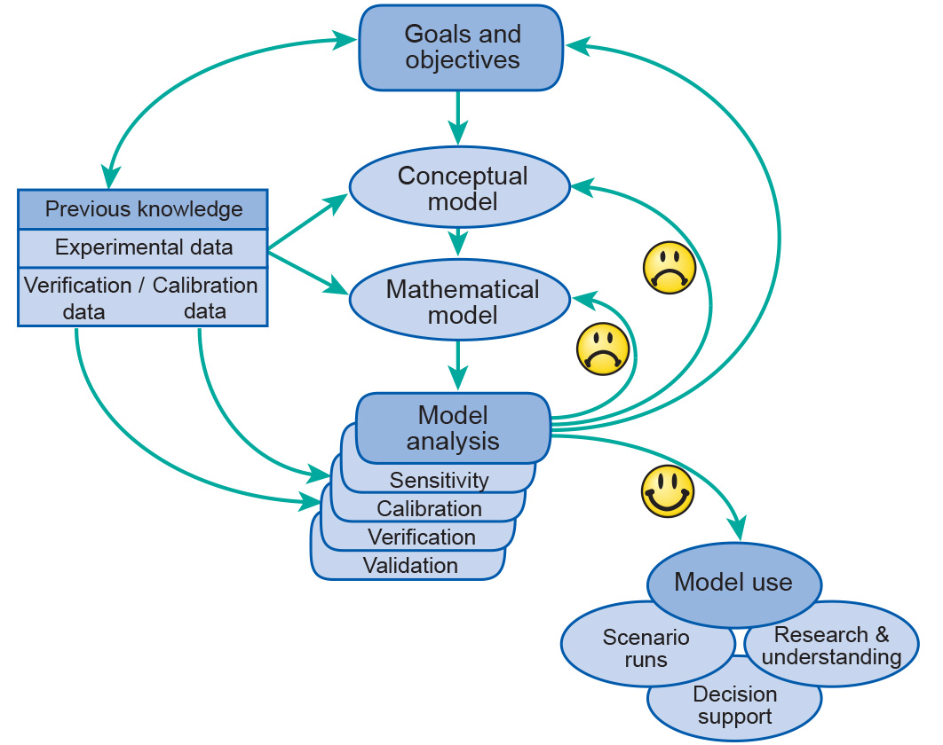
What is it that we want to find out? Why do we want to do it? How will we use the results? Who will be involved in the modelling process? Whom do we communicate the results? What are the properties of the system that need to be considered to reach the goal?

We next start looking at the information that is available about the system. This can be either data gathered for the particular system in mind, or about similar systems studies elsewhere and at other times. Note that immediately we get into the iterative mode, since once we start looking at the information available we may very quickly realize that the goals we have set are unrealistic with the available data about the system. We need to either redefine the goal, or branch out into more data collection, monitoring, observation - undertakings that may shadow the modelling effort, being much more time and resource-consuming. After studying the available information and with the goal in mind we start identifying our system in its three main dimensions: spatial, temporal and structural.

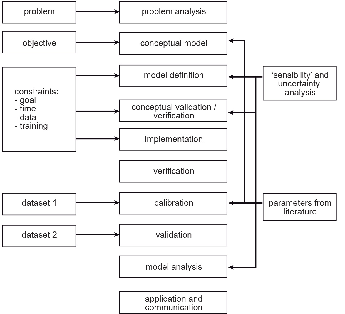
The following 10 steps (see Figure 1) may lead to the proper (mathematical) development of a model:

1. problem analysis;

2. conceptual modelling;

3. model formulation;

4. conceptual validation;

5. model implementation;

6. verification;

7. calibration;

8. validation;

9. analysis; and

10. model use, communication and evaluation.

When building a model the following questions could be useful for exploring the model’s general specifications/attributes:

• what is the problem to be modelled? (e.g. inaccessibility of a city centre);

• what are the important phenomena? (e.g. road congestion, urban land use);

• what is the spatial domain? (e.g. a built-up area of a city);

• what is the temporal domain? (e.g. morning peak-hour);

• what is the desired accuracy? Depending on the type of use, more- or less-detailed modelling (e.g in terms of spatial resolution) may be needed.

Operationalization

In the second phase, modelling concept and modelling are implemented, perhaps using commercially-available software. Functional and technical design, software validation, user-interface development, etc., are addressed. The compilation of a manual with a detailed description of the underlying model, including metadata, belongs in the operationalization process.

For operational use of the model, other questions are also relevant, such as:

• who is going to use the model (the problem owner?); and

• what resources are available for building the model (time, money).

Application

In the third phase, the model is used for calculations, simulations or making predictions within the context of the problem that had to be solved in the first place.

In total, the modelling process therefore entails the following activities: problem analysis (including area demarcation; schematic representation of processes; choice of modelling type and strategy; data collection, model development; and model calibration and verification. Sensitivity and uncertainty analysis, model presentation and visualization, and, finally, model communication may also be part of this process.