Feature Space
Introduction
A digital image is a 2D array of pixels. The value of a pixel, i.e. its DN, is in the case of an 8-bit record in the range 0 to 255. Each DN corresponds to the EM radiation reflected or emitted from a ground resolution cell—unless the image has been resampled. The spatial distribution of the DNs defines the image or image space. A multispectral sensor records the radiation from a particular GRC in different channels according to its spectral band separation. A sensor recording in three bands yields three pixels with the same row and column tuple (i, j) since they stem from one and the same GRC.
Explanation
When we consider a two-band image, we can say that the two DNs for a GRC are components of a two-dimensional vector [v1,v2],the feature vector. An example of a feature vector is [13, 55], which indicates that the conjugate pixels of band 1 and band 2 have the DNs 13and 55.This vector can be plotted in a two-dimensional graph.

Similarly, we can visualize a three-dimensional feature vector [v1,v2,v3] of a cell in a three-band image found in a three-dimensional graph. A graph that shows the feature vectors is called a feature space, or feature space plot or scatter plot. Figure 1 illustrates how a feature vector (related to one GRC) is plotted in the feature space for two and three bands. Two-dimensional feature-space plots are the most common.
Note that plotting the values is difficult for a four- or more-dimensional case, even though the concept remains the same. A practical solution when dealing with four or more bands is to plot all possible combinations of two bands separately. For four bands, this already yields six combinations: bands 1 and 2, 1 and 3, 1 and 4, bands 2 and 3, 2 and 4, and bands 3 and 4.
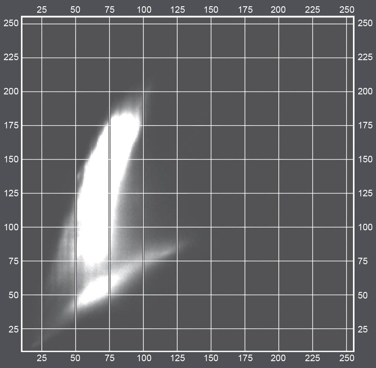
Plotting all the feature vectors of a digital image pair yields a 2D scatterplot of many points. A 2D scatterplot provides information about pixel value pairs that occur within a two-band image (Figure 2). Note that some combinations will occur more frequently, which can be visualized by using intensity or colour.
Outgoing relations
- Feature Space is defined by Image
- Feature Space is used by Class separability
- Feature Space is used by Supervised Image Classfication Algorithm