Filtering
Introduction
A further step in producing optimal images for interpretation is to apply filtering. Filtering is usually carried out for a single band. Filters - algorithms - can be used to enhance images by, for example, reducing noise (“smoothing an image”) or sharpening a blurred image. Filter operations are also used to extract features from images, e.g. edges and lines, and to automatically recognize patterns and detect objects. There are two broad categories of filters: linear and non-linear filters.
Explanation
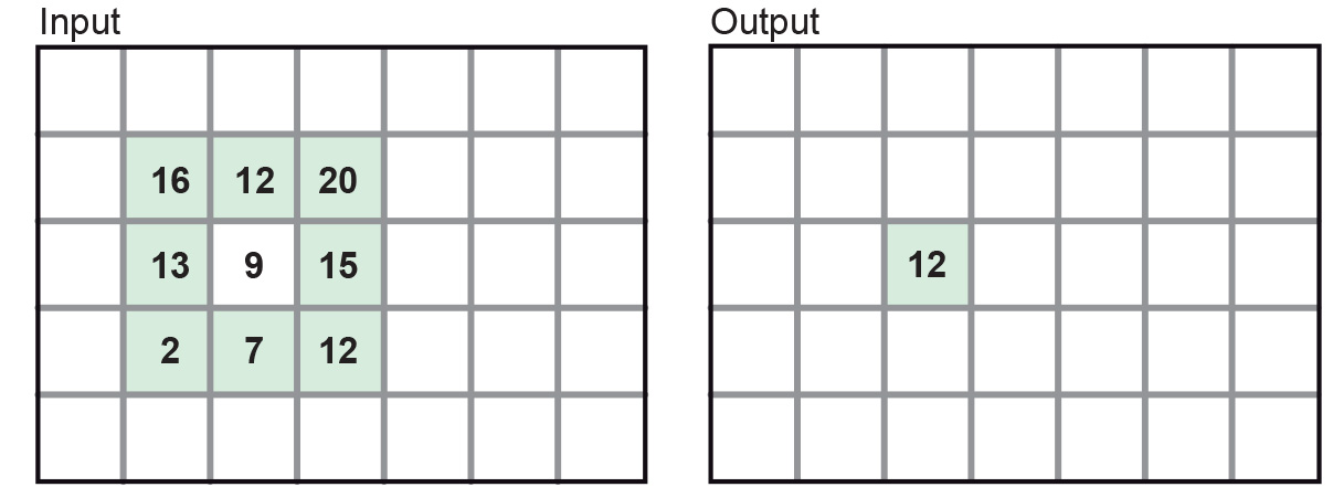
Linear filters calculate the new value of a pixel as a linear combination of the given values of the pixel and those of neighbouring pixels. A simple example of the use of a linear smoothing filter is when the average of the pixel values in a 3×3 pixel neighbourhood is computed and that average is used as the new value of the central pixel in the neighbourhood (see Figure 1).

We can conveniently define such a linear filter through a kernel.
| 1 | 1 | 1 |
| 1 | 1 | 1 |
| 1 | 1 | 1 |
The kernel specifies the size of the neighbourhood that is considered (3×3, or 5×5, or 3×1, etc.) and the coefficients for the linear combination. Image processing software allows us to select a kernel from a list or define our own kernel. The sum of the coefficients for a smoothing filter should be 1, otherwise an unwanted scaling of DN values will result.
The filtering software will usually calculate the gain:
and multiply the kernel values with it. Since there is only one way of using the kernel of a linear filter, the kernel completely defines the filter. The actual filter operation is to “move the kernel over the input image” line by line, thus calculating for each pixel a local combination of pixel values.
Although often small neighbourhoods of 3×3 kernels are considered, in practice other kernel dimensions may be used.
Prior knowledge
Outgoing relations
- Filtering is a kind of Image enhancement
Incoming relations
- Edge detection is a kind of Filtering
- Edge enhancement is a kind of Filtering
- Noise reduction is a kind of Filtering
- Local contrast enhancement is same as Filtering