Interpolation
Introduction
Interpolation is used to create a GIS layer out of point observations on a continuous variable. The reason for doing this could be manifold: for visualization purposes, for making a proper reference with other data, or for making a combination of different layers.
Explanation
Consider the problem of obtaining Y(x0), i.e. the value of a variable Y(x) at an unvisited location x0. A basic fact is Tobler’s law. This already implies intuitively that it is highly unlikely that all the predictions are equal to the mean value: deviations from the mean are likely to occur, especially in the neighbourhood of largely deviating observations. If an observation is above the regression line, then it is highly likely that observations in its neighbourhood will be above this line as well.
We will focus attention on linear combinations of the observations that we will call a predictor for Y(x0). Hence, each observation is assigned a weight such that the predictor is without bias (i.e. the predictor may yield too high a value or too low a value, but on the average it is just right). Carrying out predictions is never precise, and the difference between the value of the variable had we observed it and its interpolated value is called the prediction error. We are interested in predictions that have the lowest variance of the prediction error.
Let the optimal predictor be denoted with . It is linear in the observations, therefore
with as yet unknown weight λi. For the prediction error it is assumed that its expectation is zero
and that its variance among all linear unbiased predictors:
is minimal. The variance of the prediction error is of importance and is to be calculated below; see equation 3.
Predicting requires knowledge of the variogram. Suppose, therefore, that there are n observations, that a variogram has been determined, that a model has been fitted, and that its parameters have been estimated. The variogram values can be determined for all distances between all pairs of points consisting of observation points (which are in number). They are contained in the, symmetric, n×n matrix G. The elements of G,
, are then filled with the values obtained from
; gii contains the variogram for the distance between xi and xi, a pair of points with distance equal to zero, and hence
;
for
contains the variogram value for the distance between xi and xj and is equal to gij. The variogram can also be determined for all pairs of points consisting of an observation point and the prediction location (which are n in number). These are contained in the vector g0. The ith element of g0 contains the variogram value for the distance between xi and the prediction location x0. We first estimate the spatial mean
by means of the generalized least squares estimator
where y is the vector of observations and 1n is the vector of n elements, all equal to 1, and T denotes the transpose of a vector (or matrix). Notice that it is different from the average value, as it essentially includes the spatial dependence.
Equation 3 can be further modified as
The equation consists of two terms: the spatial mean and the term
. This second term expresses the influence on the predictor of the residuals
of the observations y with respect to the mean value
. The residuals are transformed with
.
Such a transformation is clearly based upon the variogram. Variogram values among the observation points are in cluded in the matrix G, variogram values between the observation points and the prediction location in the vector g0. Predicting an observation in the presence of spatially dependent observations is termed Kriging, named after the first practitioner of these procedures, the South African mining engineer Daan Krige, who did much of his early empirical work in the Witwatersrand gold mines.
Every prediction is associated with a prediction error. The prediction error itself cannot be determined, but an equation for the variance of the prediction error is given by
where xa equals and
.
All matrices and vectors can be filled on the basis of the data, the observation locations and the estimated variogram. We remark that the variance of the prediction error depends only indirectly upon the observations: the vector y is not included in the equation. However, the variogram is estimated on the basis of the observations, and hence the observations appear in an indirect way in the equation. The configuration of the nn observation points and the one prediction location influences the prediction error variance as well.
If a map has to be constructed of a spatial property for which the observations are collected in a 2-dimensional space the following procedure may be used:
-
Determine the empirical variogram;
-
Fit a variogram to the empirical variogram;
-
Predict values at the nodes of a fine-meshed grid;
-
Present the results in a two- or a three-dimensional perspective by linking individual predictions with line elements.
In addition to the map itself, it may be desirable (and sometimes even necessary) to display the prediction error variance (or its square root), which is obtained at the same nodes of the fine-meshed grid as the predictions themselves. This map displays the spatial uncertainty of the map.
In the manner described above, it is possible to jointly make two layers in a GIS by spatial interpolation of point observations. Such interpolation has the property that it is driven by the spatial variability of the continuous variable and is, hence, specific for each variable.
Examples
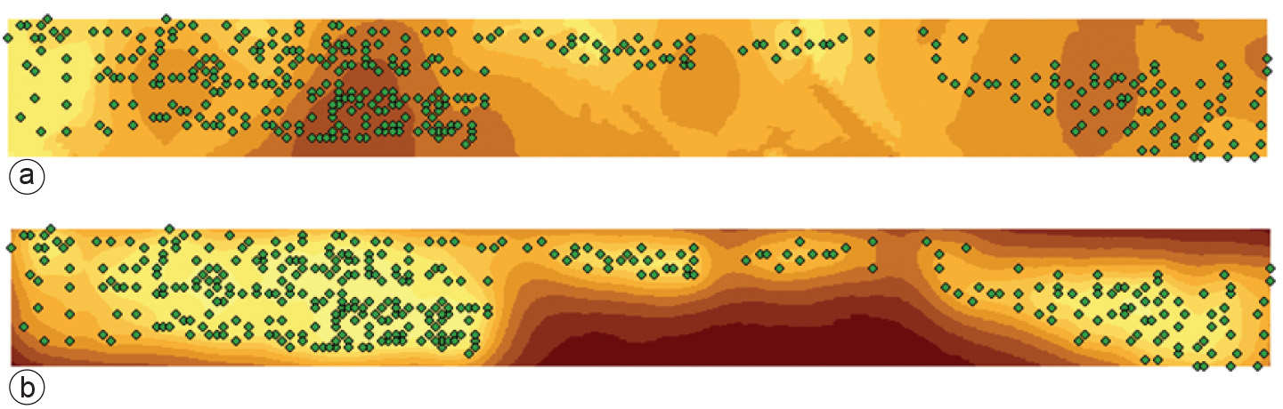
To illustrate that we consider an example. In the city of The Hague a soil inventory was carried out within an area of 2 km by 200 m (Figure above), bordering a railway. This inventory followed the closing of a cable factory in the area, and the decision making on the intended future use of the area. In total some 500 observations were provided on several chemical constituents of the possibly contaminated soil. One of the critical constituents is the the amount of lead (Pb) that was sampled from the top 50~cm of the soil. In order to get a full overview of the spatial variation of this variable, a variogram was constructed and two maps were produced: the kriged map of the Pb contamination in the soil (Figure a), and a map of the standard deviation of the prediction error (Figure b). The top map showed a large spatial variation, from peak values up to 2900~ppm (parts per million, equivalent to 2.9~g Pb per kg soil), and critical environmental thresholds were exceeded. Such heavily polluted soils have to be cleaned, in particular if the future use of the area would be residential. The kriging standard deviation showed less variation in absolute values, but it shows relatively low values close to observation locations, and increasing values at locations that are farther away from the sampling locations.
Outgoing relations
- Interpolation is based on Spatial Autocorrelation
Incoming relations
- Tessellation is produced by Interpolation